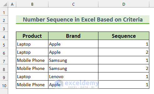
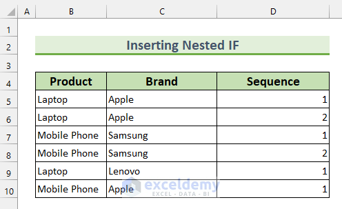
To demonstrate our methods, we have selected a dataset with 3 columns consisting of “Product,” “Brand,” and “Sequence.” The sequences will be based on the uniqueness of product-brand combos. For example, for the mobile phone, this counter resets to 1 since both items are unique.
Method 1 – Using the COUNTIF Function to Create a Number Sequence in Excel Based on Criteria
Steps:
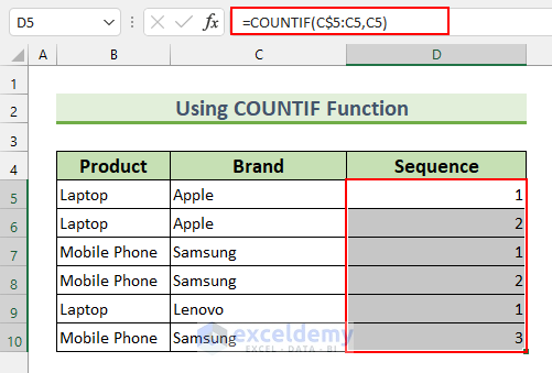
- Select the cell range D5 and use the following formula.
=COUNTIF(C$5:C5,C5)
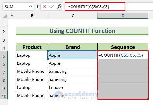
- Press Ctrl + Enter. This will AutoFill the formula to the selected cells.
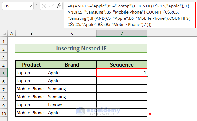
Method 2 – Inserting a Nested IF Function to Create a Number Sequence in Excel Based on Criteria
Steps:
- Use the following formula in cell D5.
=IF(AND(C5="Apple",B5="Laptop"),COUNTIF(C$5:C5,"Apple"),IF(AND(C5="Samsung",B5="Mobile Phone"),COUNTIF(C$5:C5,"Samsung"),IF(AND(C5="Apple",B5="Mobile Phone"),COUNTIFS(C$5:C5,"Apple",B$5:B5,"Mobile Phone"),1)))
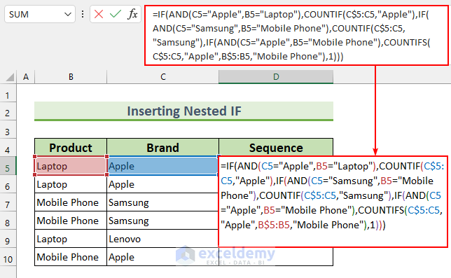
- Press Enter.
- Use the Fill Handle to AutoFill the formula to the rest of the cells.
Formula Breakdown
- There are three combined IF AND functions inside this formula. Whenever the condition is True, the formula executes the COUNTIF portion.
- AND(C5=”Apple”,B5=”Laptop”)
- Output: True.
- At first, this portion checks whether the values from cells C5 and B5 match our defined strings. If matches then it will return True.
- COUNTIF(C$5:C5,”Apple”)
- Output: 1.
- Secondly, this portion counts the number of Apple brands in the expandable range.
- COUNTIFS(C$5:C5,”Apple”,B$5:B5,”Mobile Phone”)
- Output: 0.
- Thirdly, this function counts the number of Apple mobile phones in the expandable range.
- Lastly, we have put 1 at the end of this formula that will be returned if nothing is True.
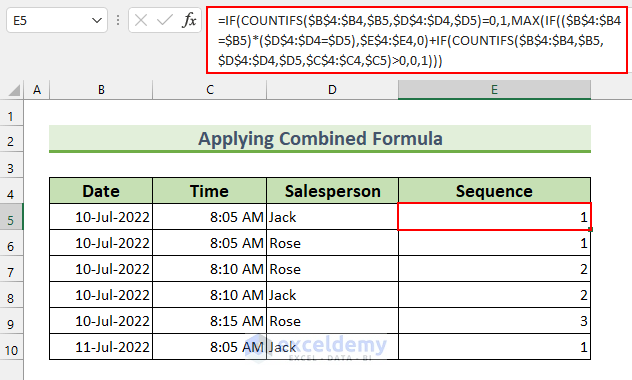
Method 3 – Applying a Combined Formula to Create a Number Sequence Based on Multiple Criteria
In this example, we will assign a number sequence for the Date, Time, and Salesperson. Different Dates will restart the number sequence.
Steps:
- Use the following formula in cell D5.
=IF(COUNTIFS($B$4:$B4,$B5,$D$4:$D4,$D5)=0,1,MAX(IF(($B$4:$B4=$B5)*($D$4:$D4=$D5),$E$4:$E4,0)+IF(COUNTIFS($B$4:$B4,$B5,$D$4:$D4,$D5,$C$4:$C4,$C5)>0,0,1)))
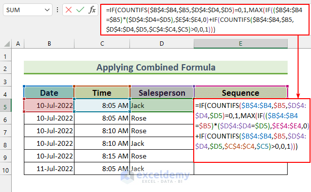
- Press Enter and AutoFill the formula.
Formula Breakdown
- There are two COUNTIFS functions inside this formula.
- The first one is → COUNTIFS($B$4:$B4,$B5,$D$4:$D4,$D5)
- Output: 0.
- This function counts the dynamic range with the same time and same salesperson.
- The second one is → COUNTIFS($B$4:$B4,$B5,$D$4:$D4,$D5,$C$4:$C4,$C5)
- Output: 0.
- Again we get a zero. This time the formula counts the dynamic range for columns B, C, and D.
- ($B$4:$B4=$B5)*($D$4:$D4=$D5)
- Output: 0.
- Here 1 means True and 0 means False. It has given us the False value.
- Our formula reduces to → IF(0=0,1,MAX(IF(0,$E$4:$E4,0)+IF(0>0,0,1)))
- Output: 1.
- We get this from the first part of the IF function as the condition is True, so we get the output as 1.
Read More: Auto Serial Number in Excel Based on Another Column
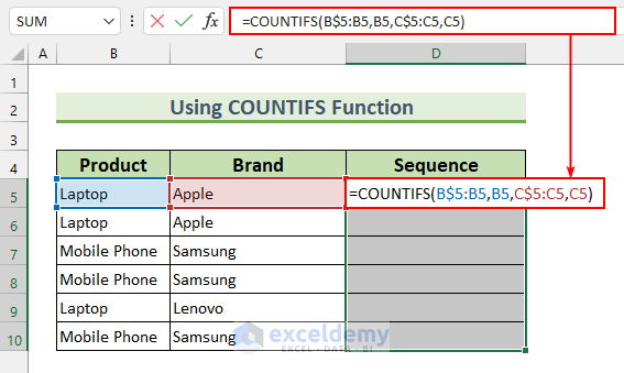
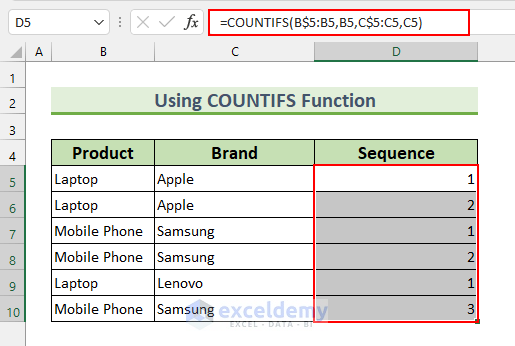
Method 4 – Using the COUNTIFS Function to Create a Number Sequence Based on Criteria
Steps:
- Select the cell range D5:D10 and insert the following formula.
=COUNTIFS(B$5:B5,B5,C$5:C5,C5)
There are two conditions in this formula. The first one looks for the product type and the second one looks for the brand name. Now, whenever these two match, the formula increments the number and thus creates a number sequence based on criteria.
- Press Ctrl + Enter. This will AutoFill the formula to the selected cells.
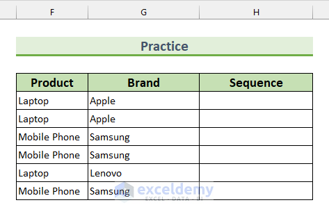
Practice Section
We have added a practice dataset for each method in the Excel file.
Download the Practice Workbook
Related Articles
- How to Perform Numbering in One Cell in Excel
- How to Add Numbers 1 2 3 in Excel
- How to Create a Number Sequence with Text in Excel
- How to Increment Row Number in Excel Formula
- Subtotal Formula in Excel for Serial Number
<< Go Back to Serial Number in Excel | Numbering in Excel | Learn Excel
Get FREE Advanced Excel Exercises with Solutions!
