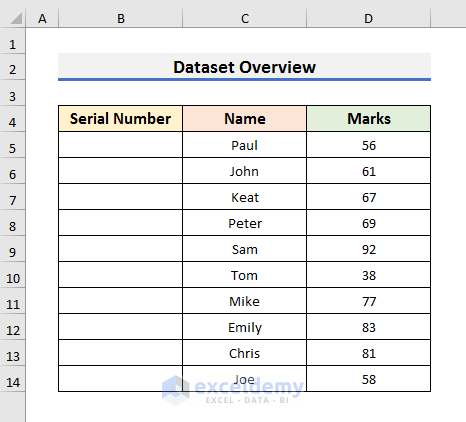
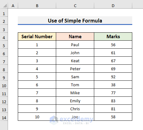
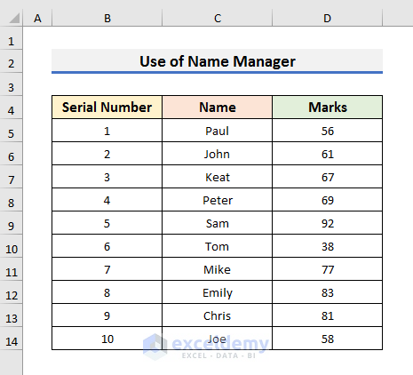
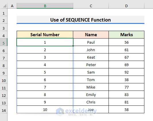
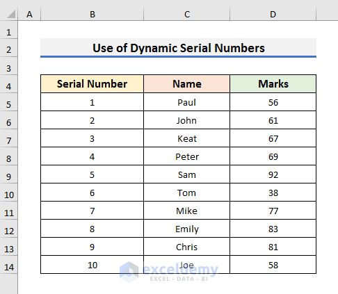
We will use a dataset that contains information about the Marks of some students. We will add automatic serial numbers to the dataset using some formulas.
Method 1 – Apply a Simple Formula to Add Automatic Serial Numbers in Excel
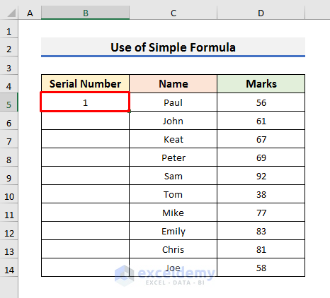
STEPS:
- Type 1 in Cell B5.
- Select Cell B6 and insert the formula below:
=B5+1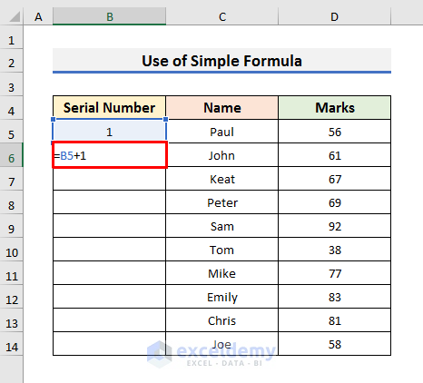
We are adding 1 to the previous cell value to get the serial numbers automatically. That’s why we need the first entry to be done manually.
- Press Enter and drag the Fill Handle down.
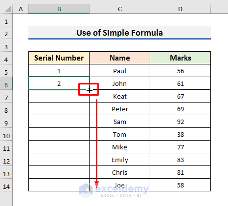
- You will see serial numbers like the below picture.
Method 2 – Adding Automatic Serial Numbers with the ROW Function
STEPS:
- Select Cell B5 and use the formula below:
=ROW()-ROW($B$4)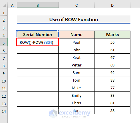
In this formula, we have used the ROW function. If you type =ROW() in Cell B5, the output will be 5 because it indicates the 5th row. The output of ROW($B$4) will always be 4 because we have used absolute cell reference here. That is why we have subtracted ROW($B$4) from ROW().
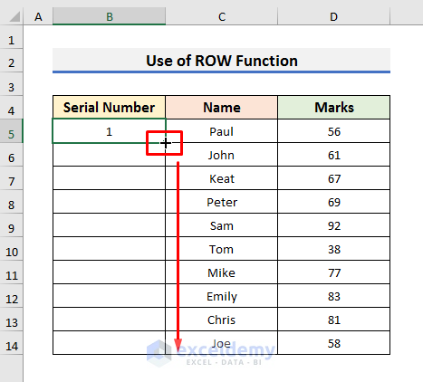
- Hit Enter and drag down the Fill Handle.
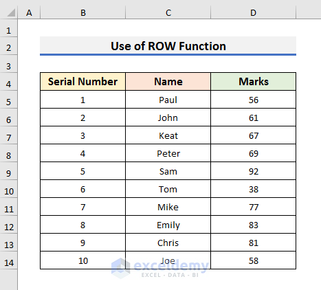
- You will see the automatic serial numbers in the dataset.
Method 3 – Using the Name Manager to Add Automatic Serial Numbers in Excel
STEPS:
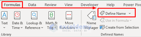
- Go to the Formulas tab and select Define Name. It will open the New Name dialog box.
- In the New Name dialog box, add a name. We have named the range as Serial.
- Use the formula below in the Refers to box:
=INDIRECT(“R[-1]C”,FALSE)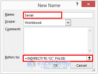
Here, we have used the INDIRECT function. The INDIRECT function returns the cell reference of a given text string. The first output of this formula is 0. It indicates the previous cell.
- Select Cell B5 and type the formula below:
=SUM(Serial,1)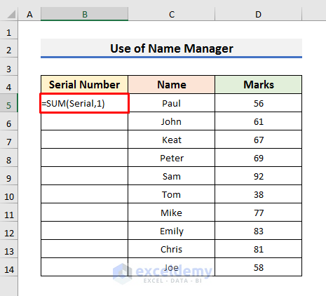
In this formula, we have used the SUM function. It sums up the value of the Serial function and 1. In the first case, the output is 1. Now, if you apply the formula in Cell B8, then, the formula will act like =SUM($B$7,1). That means it will sum up the value of Cell B7 with 1 and show it in Cell B8.
- Hit Enter and drag the Fill Handle down.
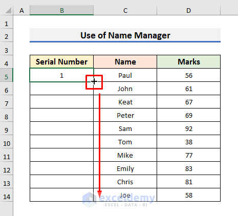
- You will see automatic serial numbers like the below picture.
Read More: How to Auto Generate Number Sequence in Excel
Method 4 – Using the COUNTA Function to Generate Automatic Serial Numbers
STEPS:
- Use the formula below in Cell B5:
=COUNTA($C$5:C5)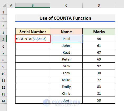
In this formula, we have used the COUNTA function to count the number of cells in the range $C$5:C5. This count will give us the serial numbers automatically. In Cell B6, the formula will change into =COUNTA($C$5:C6), which sees two values.
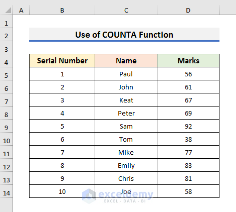
- Press Enter and drag the Fill Handle down.
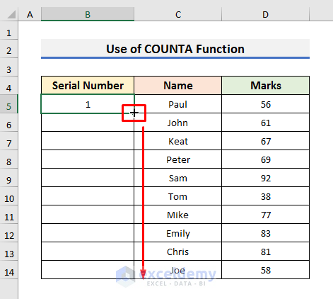
- You will be able to see the automatic serial numbers.
Method 5 – Creating Automatic Serial Numbers in Excel with the SUBTOTAL Function
STEPS:
- Select Cell B5 and use the formula below:
=SUBTOTAL(3,$C$5:C5)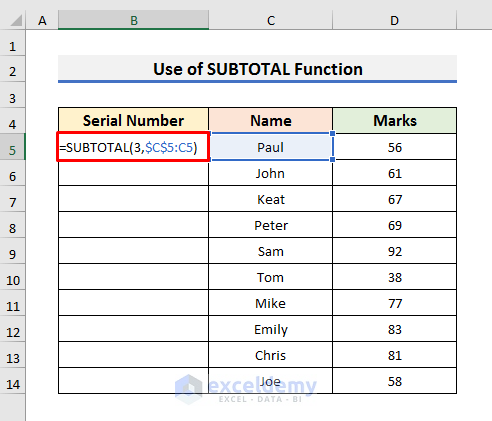
In this formula, we have used the SUBTOTAL function. The first argument indicates the function number. And function number 3 refers to the COUNTA function. So, it will count the cells in the range $C$5:C5.
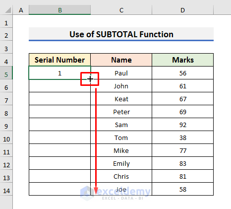
- Press Enter and drag down the Fill Handle.
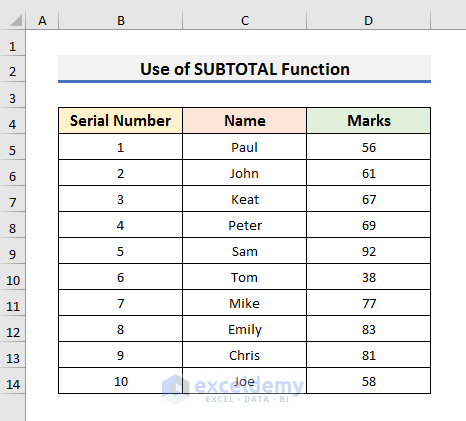
- The dataset will look like the picture below.
Method 6 – Applying the SEQUENCE Function to Add Automatic Serial Numbers with Formula in Excel
The SEQUENCE function is available in Microsoft 365.
STEPS:
- Select Cell B5 and use the following formula:
=SEQUENCE(COUNTA(C5:C14))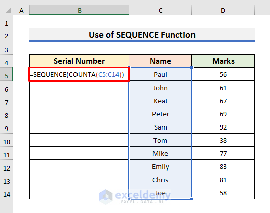
In this formula, the output of COUNTA(C5:C14) is 10. So, the formula becomes =SEQUENCE(10) after the operation of the COUNTA function. The SEQUENCE function generates a sequential list from 1 to 10.
- Hit Enter to see the results like the picture below.
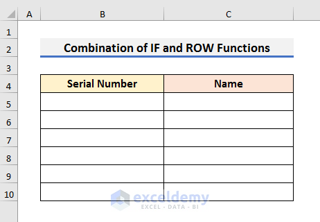
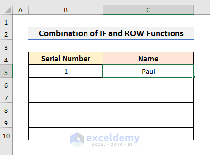
Method 7 – Combining IF and ROW Functions to Add Automatic Serial Numbers in Excel
We will add a name in Column C and the serial number will be visible automatically in Column B.
STEPS:
- Select Cell B5 and use this formula:
=IF(C5="","",ROW()-ROW($B$4))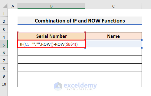
In this formula, we have used the ROW function inside the IF function. The formula will check if Cell C5 is empty or not. If Cell C5 is empty, the output of the formula will also be empty. Otherwise, it will show the value of ROW()-ROW($B$4). In the case of Cell B5, the value of ROW()-ROW($B$4) is 1.
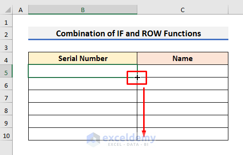
- Drag down the Fill Handle to copy the formula in the range B6:B10.
- If you type a name in Cell C5, you will see the serial in Cell B5.
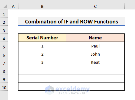
- Type a name in Cell C6 and C7, respectively, and you will get the serial numbers automatically.
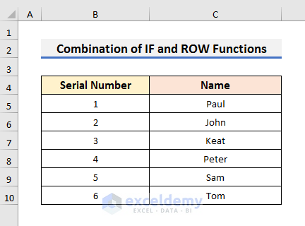
- Insert all values to get the serial numbers.
Read More: Auto Serial Number in Excel Based on Another Column
Method 8 – Using the OFFSET Function to Create Automatic Serial Numbers
STEPS:
- Insert an empty row into the dataset to avoid errors. Here, Row 5 is the added empty row.
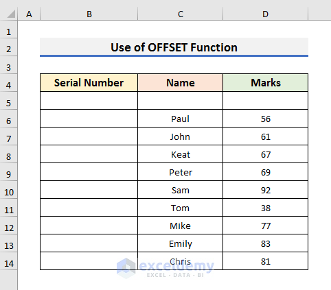
- Select Cell B6 and insert the following formula:
=OFFSET(B6,-1,0)+1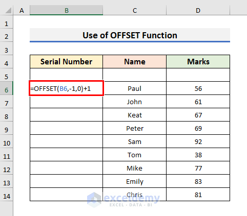
In this formula, the first argument of the OFFSET function is Cell B6. The second argument is -1 which indicates the previous row. And the third argument is 0 which refers to the same column. So, the output of OFFSET(B6,-1,0) is 0 since the Cell B5 is empty. The output of the formula is 1 for Cell B6.
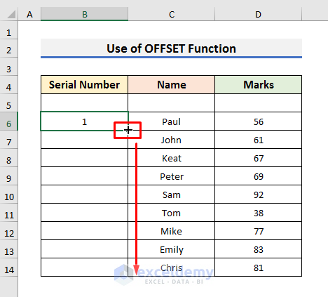
- Hit Enter and drag down the Fill Handle to copy the formula.
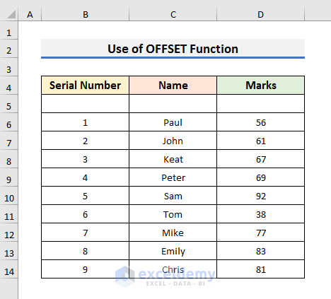
- The dataset will look like the picture below.
Read More: Auto Numbering in Excel After Row Insert
Method 9 – Adding Roman Numbers as Automatic Serial Numbers
STEPS:
- Select Cell B5 and insert the following:
=ROMAN(ROW()-ROW($B$4))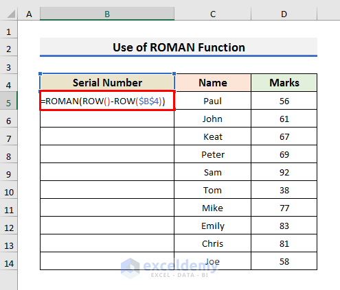
This formula is quite similar to that of Method 2. We inserted the formula of Method 2 inside the ROMAN function.
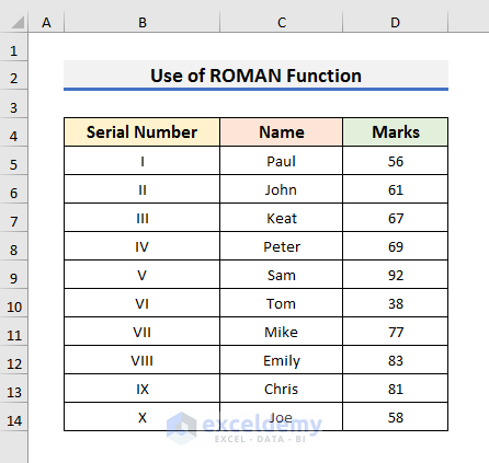
- Press Enter and drag the Fill Handle down.
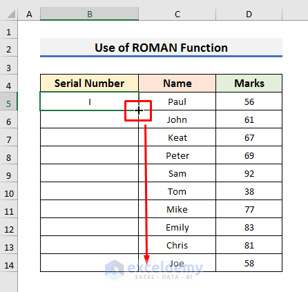
- Here’s the result.
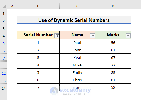
Method 10 – Adding Dynamic Serial Numbers in Excel with the Filter Option
STEPS:
- Select Cell B5 and use the formula below:
=SUBTOTAL(3,C$5:C5)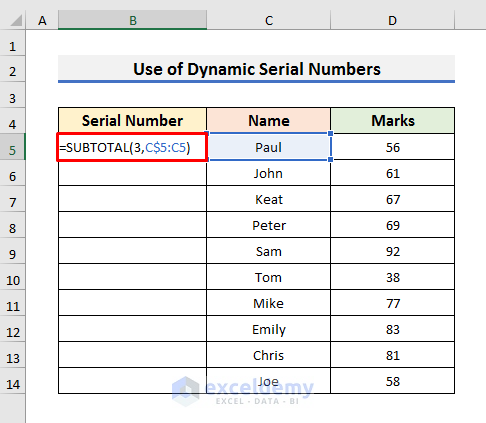
In this formula, we have used the absolute cell reference for the row index only.
- Hit Enter and drag down the Fill Handle.
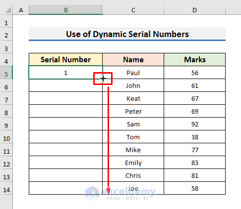
- You’ll get the serial numbers.
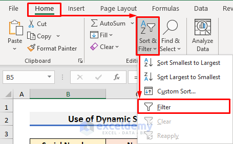
- Go to the Home tab and select Sort & Filter. A drop-down menu will appear.
- Select Filter.
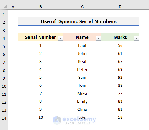
- You will see the drop-down arrows in the headers.
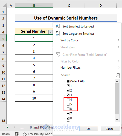
- Click on a drop-down arrow and apply the filter according to your preference. We have unchecked serial numbers 4, 5, and 6.
- Click OK to proceed.
- The filtered rows are hidden and the serial numbers are updated automatically.
Read More: Automatically Number Rows in Excel
Download the Practice Book
Related Articles
- How to Autofill in Excel with Repeated Sequential Numbers
- How to Number Columns in Excel Automatically
- Auto Generate Invoice Number in Excel
- Auto Generate Serial Number in Excel VBA
<< Go Back to Serial Number in Excel | Numbering in Excel | Learn Excel
Get FREE Advanced Excel Exercises with Solutions!
