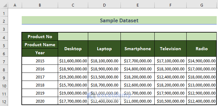
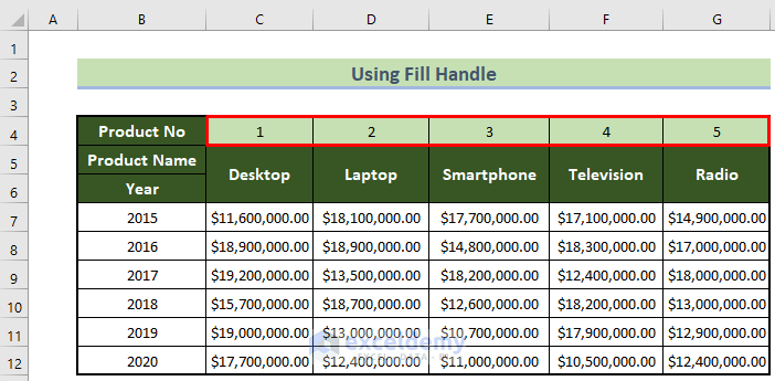
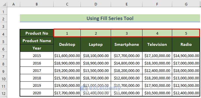
Here we have a data set with the sales record of some products for some years in a company. We’ll enter values inside the row called Product No. to number the columns.
Method 1 – Using the Fill Handle Tool to Number Columns in Excel
Steps:
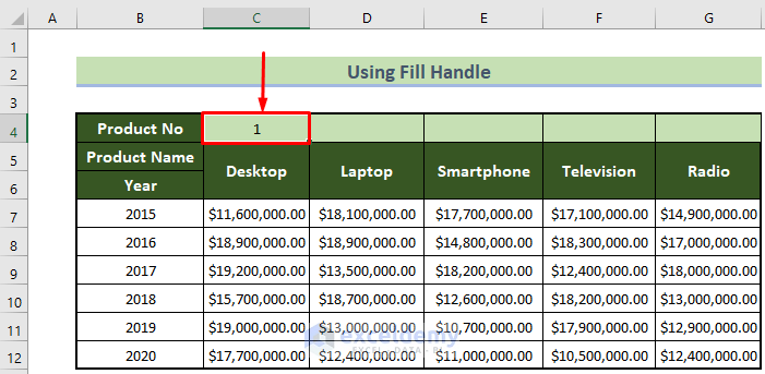
- Select the first cell (C4 here) and enter 1.
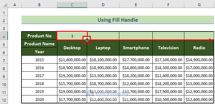
- Move your mouse cursor over the rightmost bottom corner of cell C4. You will find a small plus (+) sign. This is called the Fill Handle.
- Drag the Fill Handle right up to your last non-blank row. You will find all cells of the column get the number 1.
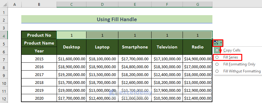
- You will find a small drop-down menu in the rightmost bottom corner of the column called Auto Fill Options. Click it.
- The Auto Fill Options drop-down menu will appear. Click on the Fill Series option.
- You will get your columns numbered automatically 1, 2, 3, …., etc.
Method 2 – Using the Fill Series Tool from the Excel Toolbar
Steps:
- Enter 1 in the first cell (cell C4 here).
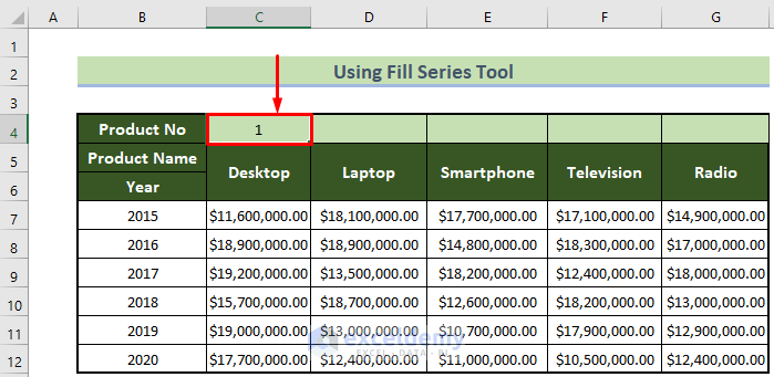
- Select the whole row.
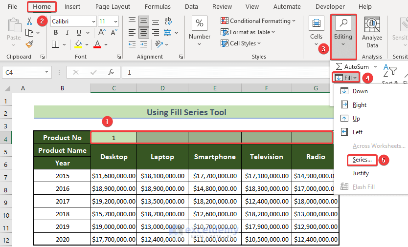
- Go to the Home tab and select the Fill option in the Excel toolbar under the section Editing.
- Click on the drop-down menu attached with the tool Fill. You will find a few options. Click on Series.
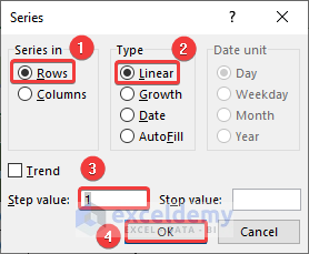
- You will get the Series dialogue box.
- From the Series in menu, select Rows.
- From the Type menu, select Linear.
- In the Step value box, enter 1.
- Click on the OK button.
- You will find your columns numbered automatically as 1, 2, 3, …, etc.
Read More: How to Auto Generate Number Sequence in Excel
Method 3 – Using Excel Functions to Automatically Number Columns
Case 3.1 – Using the COLUMN Function
Steps:
- Select the first cell (cell C4 here) and enter this formula in the Excel Formula Bar:
=COLUMN(Relative Cell Reference of the Cell)-COLUMN(Absolute Cell Reference of the Previous Cell)- In this example, it will be:
=COLUMN(B4)-COLUMN($A$4)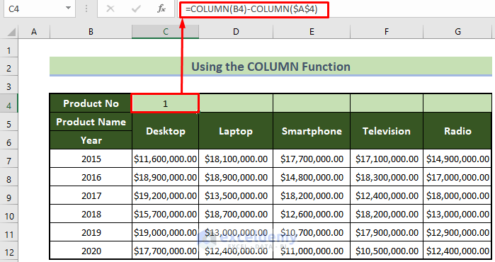
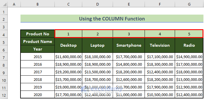
- Drag the Fill Handle right up to the last column.
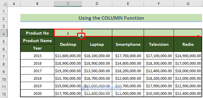
- You will find all your columns numbered.
Case 3.2 – Using the OFFSET Function
In our data set, the immediate right cell of our first cell (cell B4) is not blank, and it contains the text “Product No”.
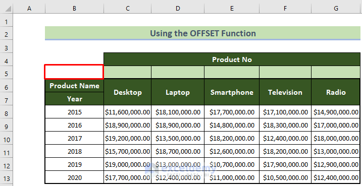
But look at the following row. Here the immediate right cell is blank. So, you can apply this function here.
Steps:
- Enter this formula in the first cell (cell C5 here):
=OFFSET(Relative Cell Reference of the Previous Cell,0,0,1,1)+1- In this example, it will be:
=OFFSET(B5,0,0,1,1)+1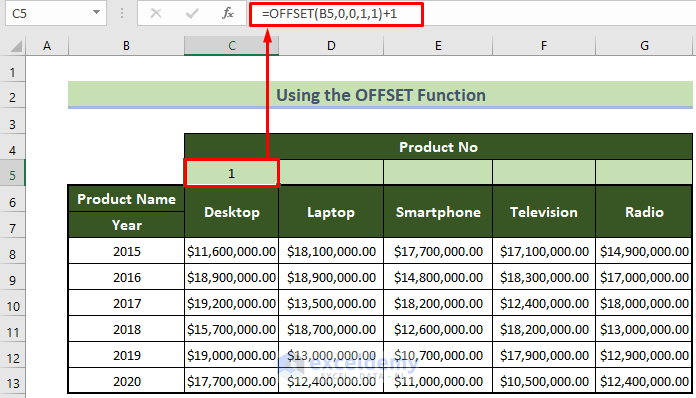
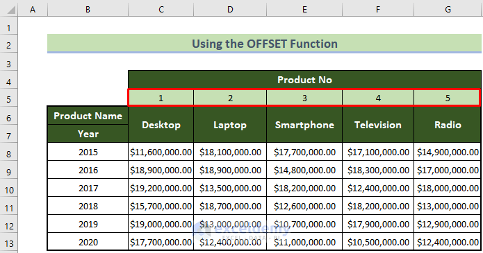
- Drag the Fill Handle right up to the last column.
- You will get all your columns numbered 1, 2, 3.
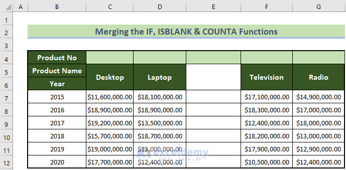
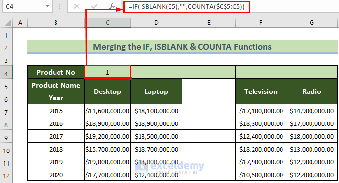
Case 3.3 – Using the IF, ISBLANK, and COUNTA Functions for Columns with Blank Cells
We have cleared the column Smartphone from the data set.
Steps:
- Enter this formula in the first cell (cell C4 here).
=IF(ISBLANK(C5),"",COUNTA($C$5:C5))Note:
C5 is the cell reference of the cell just below our first cell. You can use your one.
Formula Breakdown:
- =ISBLANK(C5)
This finds if the C5 cell is blank or not. Upon this finding, it would return TRUE or FALSE.
Result: False
- =COUNTA($C$5:C5)
This would count how many non-blank cells are in the specified range C5:C5.
Result: 1.
- =IF(ISBLANK(C5),””,COUNTA($C$5:C5))
This returns a logical operation. If the first breakdown result here is TRUE, it would return a blank cell. If the first breakdown result is FALSE, it would return the second breakdown result here.
Result: 1.
- Drag the Fill Handle right up to the last column.
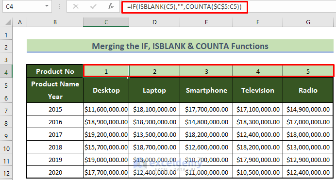
- You will get your desired result which should look like this.
Special Note:
This is a dynamic formula.
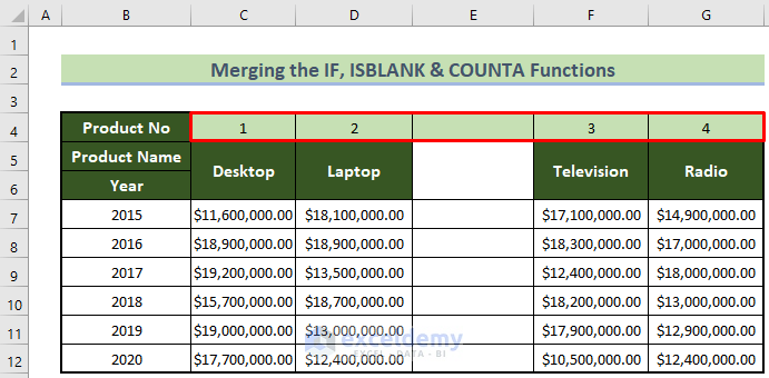
If you have a data set with all the columns non-blank, then it will number all the columns like this.
If you clear one column, it will automatically adjust and re-number them excluding the blank column.
Read More: How to Add Automatic Serial Number with Formula in Excel
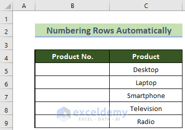
How to Number Rows Automatically in Excel
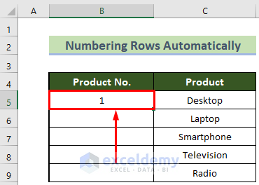
We have listed 5 products row by row.
Steps:
- Click on the first cell (cell B5 here) and insert 1.
- Place your mouse cursor in the bottom right position of the cell and drag the fill handle below.
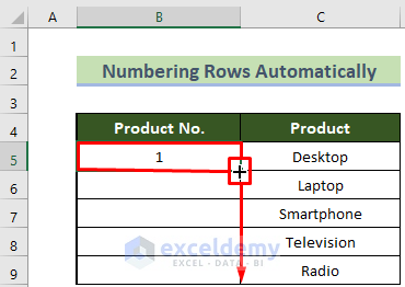
- All the cells below will now have 1 inside the cells.
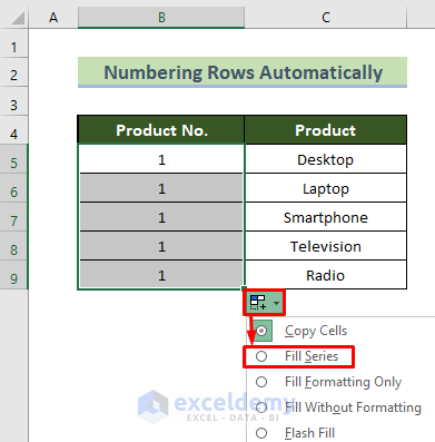
- You will find a small drop-down menu in the rightmost bottom corner of the column called Auto Fill Options. Click it.
- The Auto Fill Options drop-down menu will appear. Click on the Fill Series option.
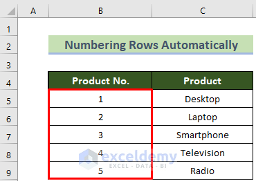
- All your rows will be numbered automatically.
Download the Practice Workbook
Further Reading
- How to Autofill in Excel with Repeated Sequential Numbers
- How to Do Automatic Numbering in Excel
- Auto Numbering in Excel After Row Insert
- Auto Serial Number in Excel Based on Another Column
- Auto Generate Invoice Number in Excel
- Auto Generate Serial Number in Excel VBA
<< Go Back to Serial Number in Excel | Numbering in Excel | Learn Excel
Get FREE Advanced Excel Exercises with Solutions!
