Automatically Number Rows in Excel (10 Easy Ways)

Although Excel does not have built-in Auto-Number features or functions, it provides various features and functions that can be used to generate auto-incremented numbers or sequential numbering in a column.

In the following video, you can see that we have automatically numbered rows in Excel.

Why Automatically Number Rows in Excel?

Organization: Automatically numbering rows makes it simpler to find and refer to specific rows.
Sorting and Filtering (Data Analysis): Numbered rows make it easy to sort and filter data effectively, particularly useful when dealing with big sets of data.
Data Entry: Removes the need for counting manually and lowers the risk of making mistakes.
Collaboration: In teamwork settings, it helps everyone have a clear and consistent way to refer to rows.
Document Control: When you make forms or templates in Excel, auto-numbering rows is helpful for keeping track of things and checking them later.

Automatically Number Rows in Excel: 10 Easy Ways

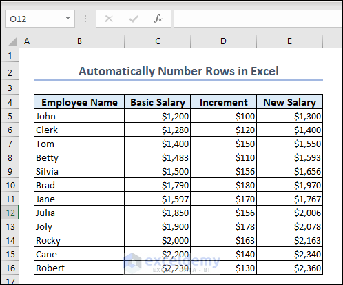
The following dataset has several rows, however there is no serial number in the rows. Using this dataset, we will go through 10 easy methods to automatically number rows in Excel.

Here, we used Microsoft 365. You can use any available Excel version.

Method 1 – Using SEQUENCE and COUNTA Functions

STEPS:

Enter the following formula in cell B5:

=SEQUENCE(COUNTA(C:C)-1)

Press ENTER,

The rows are automatically numbered according to their serial number.

Formula Breakdown

SEQUENCE(COUNTA(C:C)-1)

COUNTA(C:C): Counts the number of non-empty cells in column C.
COUNTA(C:C)-1: Subtracts 1 to exclude the header cell from the count.
SEQUENCE(COUNTA(C:C)-1): Generates a sequence of numbers based on the specified parameters. In this case, it will create a sequence starting from 1 and ending at the value obtained in step 2 (the count minus 1). Each number in the sequence will increment by 1.

Method 2 – Using VBA Code

Generating an auto serial number using VBA macros is an effective method when dealing with a larger dataset.

STEPS:

Go to the Developer tab >> select Visual Basic.
Alternatively, press the ALT+F11 keys.

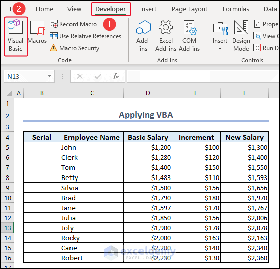
A VBA Editor window will appear.

From the Insert tab >> select Module.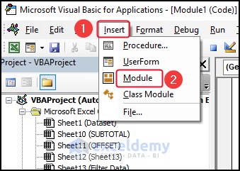

Enter the following VBA code in the Module:

Sub AUTOMATIC_ROW_NUMBER()
Dim row_range As Range, data_range As Range, c As Long
B = 1
Set data_range = Range("C5:C" & Range("C" & Rows.Count).End(xlUp).Row)
       For Each row_range In data_range.SpecialCells(xlCellTypeVisible)
                row_range(1, 0).Value = B
                B = B + 1
       Next row_range
End Sub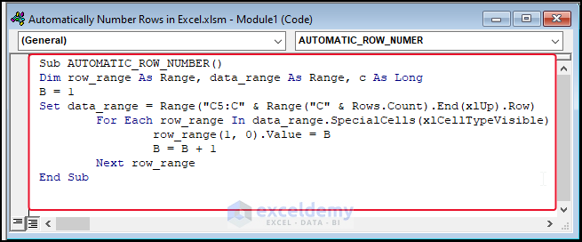

Code Breakdown

Sub AUTOMATIC_ROW_NUMBER()

Defines the start of a subroutine named AUTOMATIC_ROW_NUMBER.

Dim row_range As Range, data_range As Range, c As Long

Declares three variables: row_range, data_range, and c.
row_range and data_range are declared as Range objects, which can hold a range of cells.
c is declared as a Long data type, which can store large integer values.

B = 1

Assigns the value 1 to a variable named B.
Initializes B as the starting value for numbering the rows.

Set data_range = Range(“C5:C” & Range(“C” & Rows.Count).End(xlUp).Row)

Sets the data_range variable to a range of cells from C5 to the last non-empty cell in column C.

For Each row_range In data_range.SpecialCells(xlCellTypeVisible)

Starts a For…Next.. loop that iterates through each cell in the data_range variable.
SpecialCells(xlCellTypeVisible) filters the range to only include visible cells, excluding any hidden or filtered cells.

row_range(1, 0).Value = B

Assigns the value of B to the cell in the current row of the row_range.
row_range represents a single cell within the data_range.

B = B + 1

Increments the value of B by 1, preparing it for the next row.

Next row_range

Marks the end of the loop.

End Sub

Ends the Sub.

Run the code by pressing F5, and the rows get serial numbers automatically.

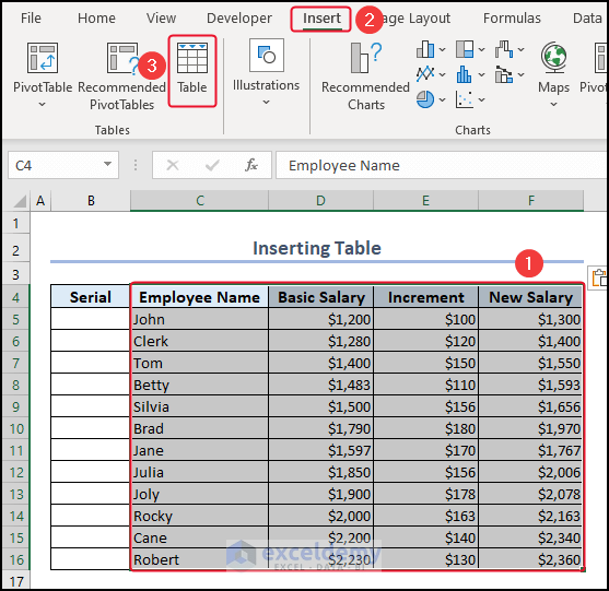
Method 3 – Inserting Table and Using ROW Function

After creating a Table from our dataset, we will use the ROW function to automatically number rows in Excel.

STEPS:

To insert a Table, select the range of cells C4:F16, excluding the Serial column.
Go to the Insert tab.
From the Tables group, select Table.

A Create Table dialog box will appear.

Ensure My table has headers is marked.
Click OK.

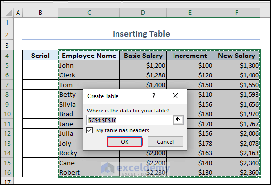
The table is created.

Enter the following formula in cell B5:

=ROW(Table2)-4

Press ENTER.

The rows get serial numbers automatically.

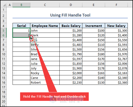
Method 4 – Using Fill Handle Feature

The Fill Handle tool is an easy way to automatically number rows in Excel.

STEPS:

Enter 1 & 2 in cells B5 and B6 respectively.
Select both of the cells (B5 and B6).

A small green-colored Square will appear at the bottom of the cells that we selected.

Move the cursor to the Square & it will turn into a black colored PLUS icon (Fill Handle).
Double-click on the PLUS.

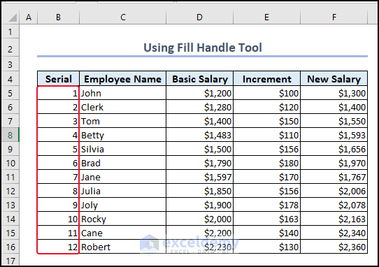
All the rows now have serial numbers.

Note: If you have data with adjacent blank entries, double-clicking on Fill Handle will not work. In this case, drag the Fill Handle down to your desired row & rows containing both blank & non-blank entries will be auto-numbered.

Method 5 – Using Fill Series Feature

Unlike Fill Handle, the Fill Series option offers various options to create a number sequence in Excel without dragging, such as Linear, Growth, Date, and Autofill.

STEPS:

Enter 1 in cell B5.
Go to the Home Tab >> Click Fill (in the Editing Section) >> Select Series (from the drop-down menu).

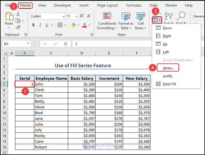
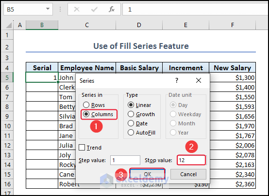
A Series dialog box will appear.

Select Columns (under Series in) & Linear (under Type).
Choose Step Value & Stop Value in the dialog box (in our case, Step Value 1, Stop Value 12).
Click OK.

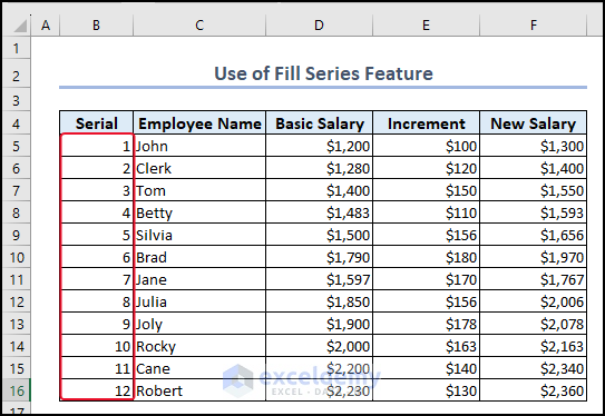
All the row numbers are auto-numbered.

Method 6 – Using ROW Function

STEPS:

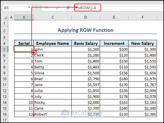
Enter the following formula in cell B5:

=ROW()-4

The ROW function finds and returns the row number of a cell reference.

Press ENTER.

the outcome is displayed in cell B5.

Drag down the formula with the Fill Handle tool.

The complete Serial column is as follows.

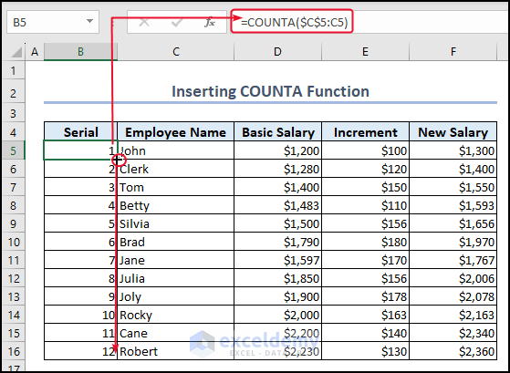
Note: The ROW Function numbers rows irrespective of adjacent row entry types. If you want to ignore blank rows,use =IF(ISBLANK(C5),””,ROW()-4) in cell B5, then drag the Fill Handle to serialize. The formula numbers blank cells without showing them.

Method 7. Using COUNTA Function

STEPS:

Enter the following formula in cell B5:

=COUNTA($C$5:C5)

The COUNTA function calculates the number of non-empty cells in a range.

Press ENTER.

The outcome is displayed in cell B5.

Drag down the formula with the Fill Handle tool:

The complete Serial column is as follows:

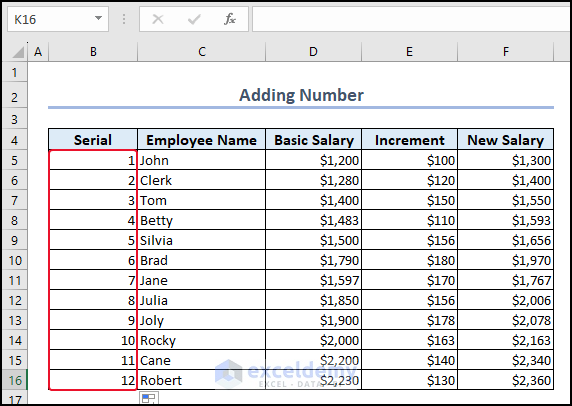
Method 8. Adding Number

Adding a number to the previous row number can display the row number as you want.

Enter 1 (or any number with which you want to start serialization) in the first row (B5).
In the 2nd row enter the following formula and press ENTER:

=B5+1

Drag the Fill Handle down to copy this formula.

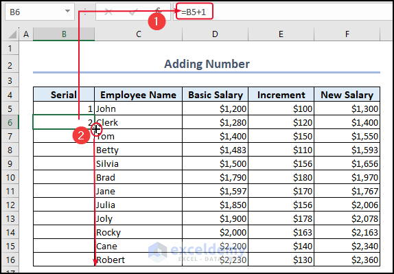
The complete Series column is numbered.

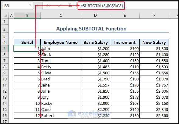
Method 9 – Using SUBTOTAL Function

STEPS:

Enter the following formula in cell B5:

=SUBTOTAL(3,$C$5:C5)

The SUBTOTAL function finds and returns the subtotal for a range of cells.

Press ENTER.

The result is returned in cell B5.

Drag down the formula with the Fill Handle tool.

The complete Serial column is as follows:

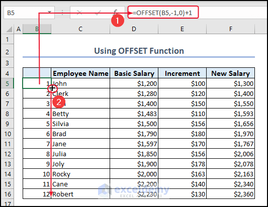
Method 10 – Using OFFSET Function

STEPS:

Enter the following formula in cell B5:

=OFFSET(B5,-1,0)+1

Press ENTER.

The result is returned in cell B5.

Drag down the formula with the Fill Handle tool.

The complete Serial column is numbered.

How to Hide or Display Fill Handle Tool in Excel

The Fill Handle tool is displayed by default. However it is possible to hide it, and conversely, unhide it if it is hidden.

STEPS:

Go to the File menu.

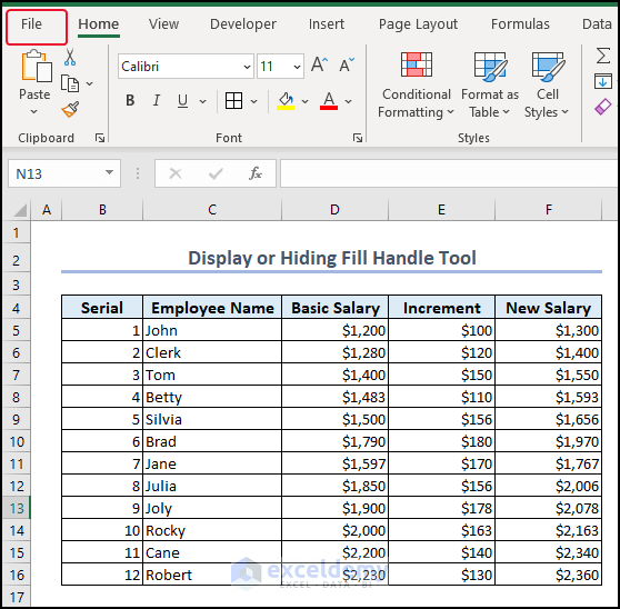
Select Options.

An Excel Options dialog box will appear.

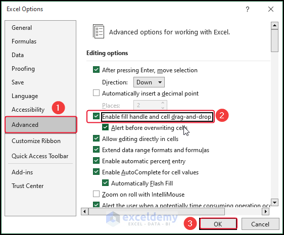
Select Advanced.
To display the Fill Handle tool, mark Enable fill handle and cell drag and drop.
Click OK.

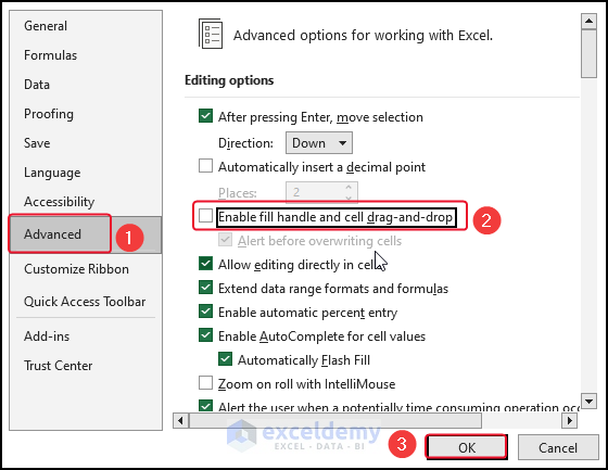
To hide the Fill Handle tool, unmark the Enable fill handle and cell drag and drop, then click OK.

Things to Remember While Using Auto-Numbered Methods

Identify Values Before Using Functions: Make sure to choose the numbers you want to begin and end with before using any function. Also, consider which method is suitable depending on how big your spreadsheet is, as larger spreadsheets can be more complicated.
Verify Your Work: Although auto-number functions can be very helpful, they are not always flawless.

Download Practice Workbook

Automatically Number Rows.xlsm

<< Go Back to Serial Number in Excel | Numbering in Excel | Learn Excel

Get FREE Advanced Excel Exercises with Solutions!

Automatically Number Rows in Excel (10 Easy Ways)

Why Automatically Number Rows in Excel?

Automatically Number Rows in Excel: 10 Easy Ways

Method 1 – Using SEQUENCE and COUNTA Functions

Method 2 – Using VBA Code

Method 3 – Inserting Table and Using ROW Function

Method 4 – Using Fill Handle Feature

Method 5 – Using Fill Series Feature

Method 6 – Using ROW Function

Method 7. Using COUNTA Function

Method 8. Adding Number

Method 9 – Using SUBTOTAL Function

Method 10 – Using OFFSET Function

How to Hide or Display Fill Handle Tool in Excel

Things to Remember While Using Auto-Numbered Methods

Related Articles

Leave a reply Cancel reply