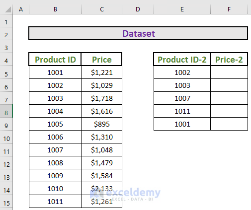
Suppose you have a simple table with two columns, and you want to make a new table that is a subset of the first one. You can do so by making a new table where the first column will have some values from the first table, and then match the corresponding values from the first table into the second one.
Let’s look into the example table, which contains some product IDs along with their corresponding prices. Then, you make another column with the heading Product ID-2. By comparing columns Product ID and Product ID-2, you can return the values from the Price column and fill them into the Price-2 column.
Method 1 – Use the VLOOKUP Function to Match Two Columns and Return a Third in Excel
The first method uses the VLOOKUP function, one of the most common lookup table tools for Excel. It fetches a value on a column a certain number of columns to the right of the value you need (the lookup value). Here’s how to utilize the function.
Steps:
- In the example sheet, select F5 and type in the following formula:
=VLOOKUP(E5,$B$5:$C$15,2,FALSE)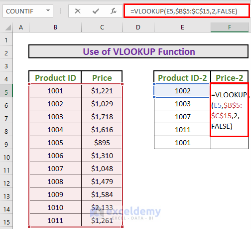
Formula Explanation:
- Here, the lookup value is E5.
- The array is B5:C15.
- The column index number is 2 (since the price is in the second column of the array).
- Excel will find the value from E5 in the column B, then return the value of the cell in column C in the same row as the result (since C is the second column of the lookup array).
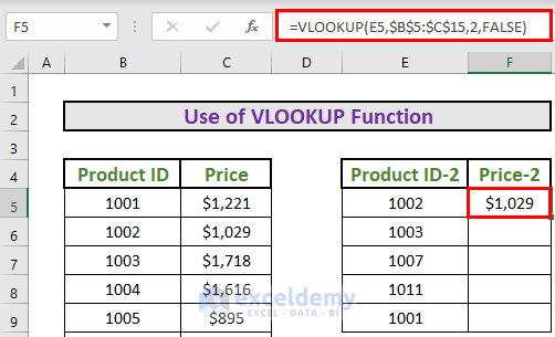
- Then, press ENTER to get the output.
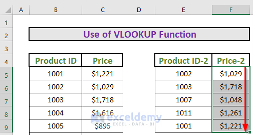
- After that, use the Fill Handle to AutoFill up to F9.
Read More: Excel formula to compare two columns and return a value
Method 2 – Combination of INDEX-MATCH Functions to Match Two Columns and Return a Third in Excel
The next method is an important one. Here, I will use a combination of the INDEX and MATCH Functions. Let’s see the steps.
Steps:
- Go to F5 and write down the following formula
=INDEX($C$5:$C$15,MATCH(E5,$B$5:$B$15))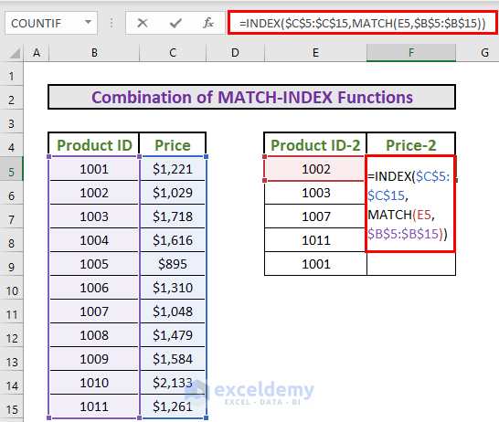
Formula Breakdown:
- MATCH(E5,$B$5:$B$15) → Excel will return the relative position 1002 in the array B5:B15.
- Output: {2}
- INDEX($C$5:$C$15,MATCH(E5,$B$5:$B$15)) → This becomes INDEX($C$5:$C$15,2)
- INDEX($C$5:$C$15,2) → Excel will find the second element in the array C5 to C15.
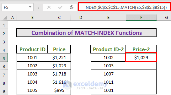
- Output: {1029}
- Now, press ENTER to get the output.
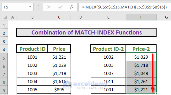
- Finally, use the Fill Handle to AutoFill from F5 up to F9.
Method 3 – Combination of IF, INDEX, and MATCH Functions to Match Two Columns and Return a Third in Excel
Let’s say that you need to compare based on two columns in the table rather than just one. For this method, the dataset needs to be changed a little bit.
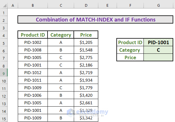
This time, the result needs to match both the Product ID and Category and get the price. A combination of the IF, INDEX, and MATCH functions will work here.
Steps:
- Go to G7 and copy the following formula:
=INDEX(D5:D15,MATCH(G5,IF(C5:C15=G6,B5:B15),0))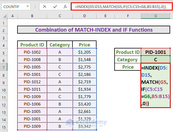
Formula Breakdown:
- C5:C15=G6 → This is the logical test for the IF The condition is an array condition.
- Output: TRUE is for Category C (since that’s the value of G6) and FALSE is for other categories. {FALSE;FALSE;TRUE;TRUE;FALSE;FALSE;TRUE;FALSE;FALSE;FALSE;FALSE}
- B5:B15 → This is the value if the test is TRUE.
- MATCH(G5,IF(C5:C15=G6,B5:B15),0)) → G5 is the lookup value and the lookup array is IF(C5:C15=G6,B5:B15), that means Excel will look for PID-1001 from {FALSE;FALSE;”PID-1005″;”PID-1001″;FALSE;FALSE;”PID-1009″;FALSE;FALSE;FALSE;FALSE} and get you the relative position.
- Output: {4}
- INDEX(D5:D15,MATCH(G5,IF(C5:C15=G6,B5:B15),0)) → This becomes
- INDEX(D5:D15,4)
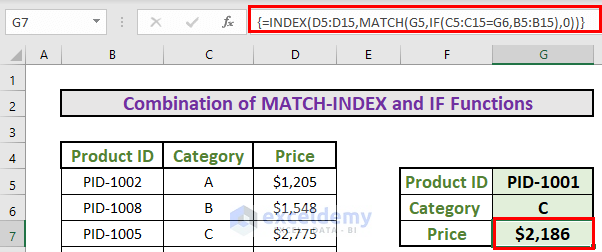
- Output: {2186}
- Then, press CTRL+SHIFT+ENTER to get the output. This is because it’s an array formula and it needs to do multiple array calculations to get a result. You will see a pair of 2nd brackets appear in the formula which contains the formula inside it.
Things to Remember
- The absolute reference is for locking a range so it doesn’t change when you copy it or drag the Drop Handle for AutoFill.
- CTRL+SHIFT+ENTER is for array formulas.
Download Practice Workbook
Download this workbook and practice while going through this article.
<< Go Back to Columns | Compare | Learn Excel
Get FREE Advanced Excel Exercises with Solutions!

the same can be done with SUMPRODUCT: SUMPRODUCT((A2:A12=F2)*(B2:B12=F3)*C2:C12)
Better formula as you can compare more than just two cell, the only downside is that it will return with “0” and not #N/A which cause an issue if you are comparing data from two different time.
Thanks, Emil!
Freat, I loved it.
Thanks.
How To Compare Two Columns with the single-cell And Return in multiple Values From The second Column In the single cell of Excel?
Hi MAHENDRA TRIVEDI! You can use the following formula to compare two columns and return multiple matches in a single cell:
=TEXTJOIN(",",TRUE,IF(A5:A15=D5,B5:B15,""))Here,
A5:A15= Range for matching criteria
B5:B15 = Range of the values to return
D5= Lookup value
TRUE ignores all the empty cells.
Check the 3rd case of the following article to know more details.
hhttps://www.exceldemy.com/index-match-return-multiple-values-vertically/
Thanks for being with us. Best regards.
I am keeping a note of your problem. Thanks.
Great work. Thanks.
Thanks, Uche.
Hi. Thanks for this. Can you use this formula when the looked up values are on a different sheet ?
If you’ve some specific problem, let us know via email, we shall try to make a blog post with your problem.
Thanks for this however when I try to run this on my data I always get a #VALUE! error on the second column range of data
https://i.imgur.com/ysJTNYR.png
Nevermind dont know what changed but I got it working. thanks again!
That’s great Griffin, I hope you get benefited from our articles.