How to Plot Least Squares Regression Line in Excel (5 Methods)

The Least Squares Regression Line – A Statistical Tool for Analyzing Relationships

The least squares regression line is a widely used statistical method for examining the relationship between two continuous variables. It can be applied in Excel to determine the best-fitting line for a given set of data points, enabling predictions of future outcomes based on historical performance. In this article, I’ll share five effective methods to plot the least squares regression line in Excel.

In the following, you will find an overview of the least squares regression line in Excel.

Understanding the Least Squares Regression Line

The term “Least Squares” refers to the approach of finding the line that minimizes the sum of squared differences between observed data points and their corresponding predicted values on the line. Essentially, it represents the average trend within the data. By using this line of best fit, we can make informed predictions about future values of the dependent variable based on the independent variable.

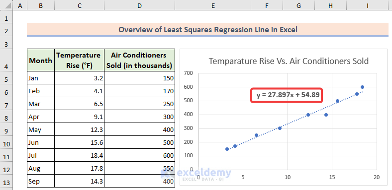
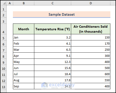
Dataset Overview

Let’s consider a hypothetical dataset with monthly records of Temperature Rise (°F) and Air Conditioners Sold (in thousands).

Method 1 – Using Scatter Chart to Plot Least Squares Regression Line

When creating a scatter chart to display a least squares regression line, follow these steps:

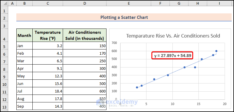
• First, plot the data points on the chart.
• Next, add the line of best fit by using the linear regression equation. Calculate the y-values for a range of x-values.
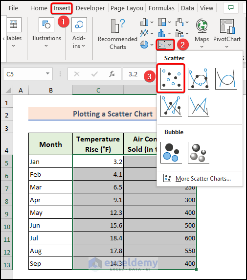
• To create the scatter chart in Excel:
  • Select the relevant columns from your table.
  • Choose the Scatter chart type from the Insert menu.

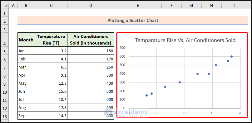
• • The scatter chart will appear within the worksheet.

• Visit the Add Trendline option from the Advanced settings.

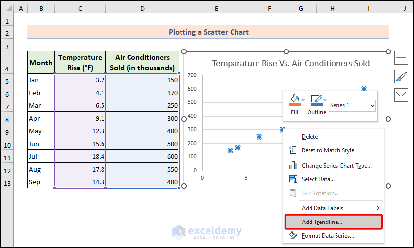
• In the right pane, checkmark the Display Equation on chart option.

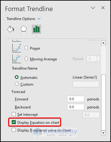
• You’ll see the least squares regression line displayed on the chart.

Method 2 – Using Arithmetic Formula to Calculate Least Squares Regression Line

The formula for calculating the least squares regression line involves basic arithmetic calculations and is straightforward to use. The regression line formula is:

ŷ = a + bx

Where,

ŷ= represents dependent variable.

x= is the independent variable.

a= is the y-intercept.

b= is the slope of the line.

To calculating the slope of the line (b) enter the following formula:

b=xy-xynx2-(x)2n

To find the y-intercept (a), enter the formula:

a=y-(bx)n

Here are the steps:

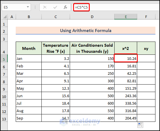
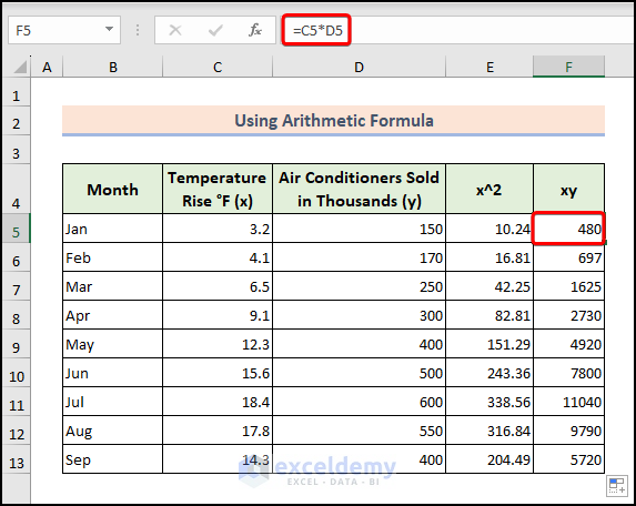
• Calculate the x^2 value in a helper column using the formula:

• • Here, C5 is the starting cell of the Temperature Rise column.

• In another helper column, compute xy using:

• • Here, D5 is the starting cell of the Air Conditioner Sold in Thousands column.

• Below the table, determine the Total Sum Value row-wise using the SUM function:

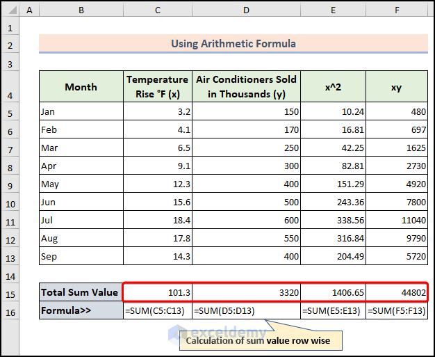
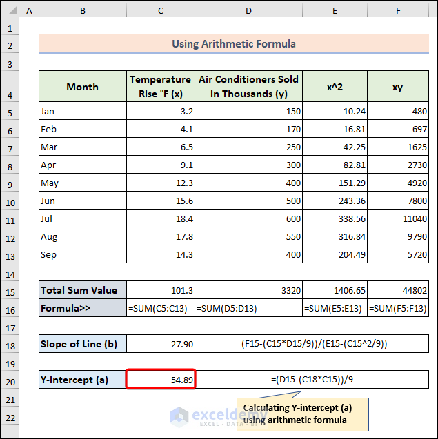
• Calculate the Slope of Line (b) using the formula:

• • Here, F15, C15, D15, and E15 cells represent sum values of Temperature Rise, Air Conditioners Sold, x^2, and xy respectively.

• Calculate the Y-intercept (a) using:

• • Here, D15, C15, and C18 cells represent sum value of Air Conditioner Sold in Thousands, Temperature Rise, and Slope of Line respectively.

• Finally, compute the least square regression line using the basic linear line formula:

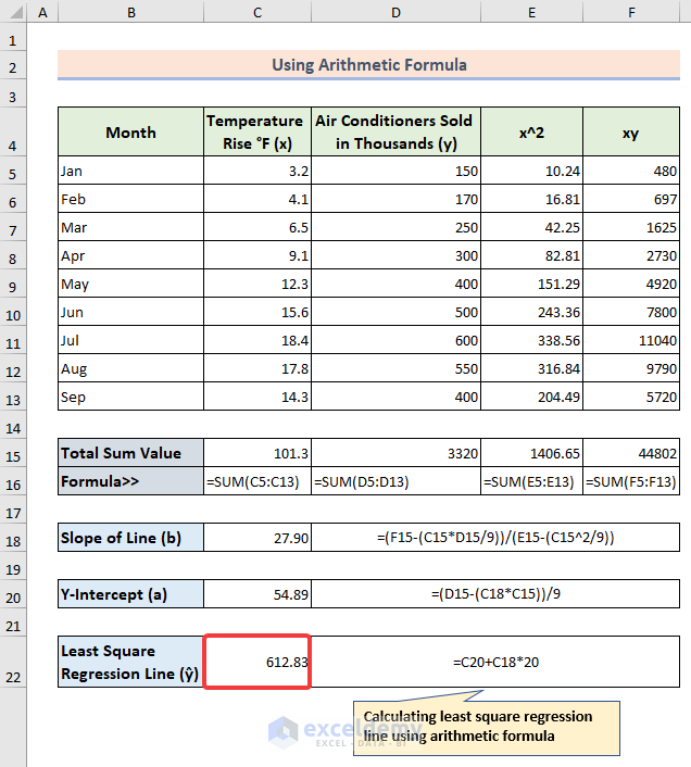
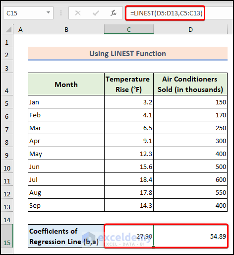
Method 3 – Using the LINEST Function to Obtain the Least Squares Regression Line

The LINEST function in Excel is a mathematical tool used to calculate the least squares regression line for a given set of data points. When you apply this function, it returns an array of values, including the slope, y-intercept, correlation coefficient, and regression statistics for the best-fitting line.

Follow these steps:

• Start by selecting a cell and applying the following formula:

• • Here, D5:D13 represents the dependent variable (e.g., Air Conditioners Sold), and C5:C13 represents the independent variable (e.g., Temperature Rise).

• Use the linear line formula to obtain the final output for the least squares regression line:

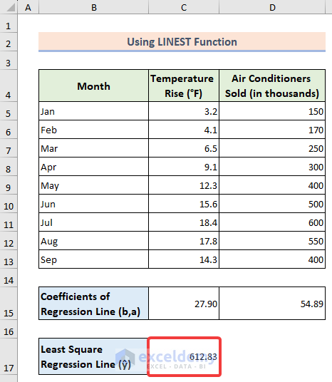
Method 4 – Combining the SLOPE and INTERCEPT Functions to for the Least Squares Regression Line

The SLOPE and INTERCEPT functions in Excel can be combined to determine the equation of the least squares regression line. Here’s how:

• Calculate the slope of the line (denoted as (b)) using the following formula:

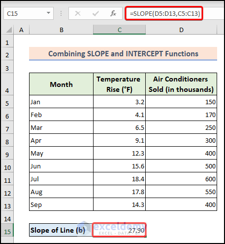
• Find the y-intercept using the INTERCEPT function:

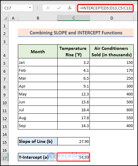
• Similar to the previous methods, use the linear line formula to get the least squares regression line value:

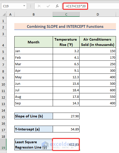
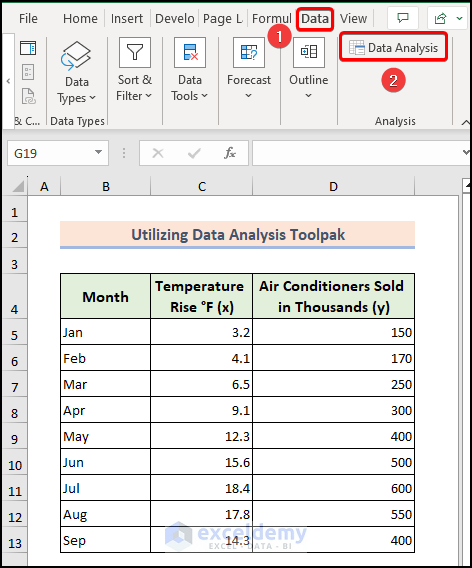
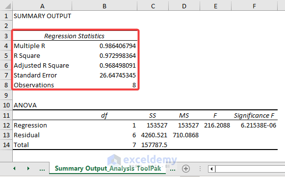
Method 5 – Utilizing the Data Analysis ToolPak for Calculating the Least Squares Regression Line

The Data Analysis ToolPak is an Excel add-in that provides various statistical tools, including regression analysis. Follow these steps:

• While in the worksheet, click the Data Analysis option from the Data tab.

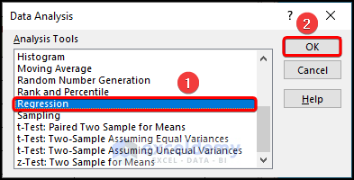
• In the Data Analysis window, choose Regression and click OK.

• Select the desired range of cells and checkmark the Labels and Residuals options. Click OK.

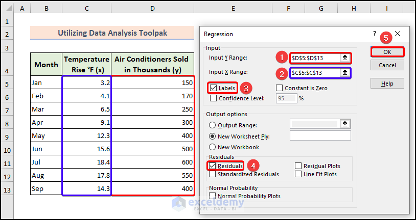
• A new worksheet will open, displaying regression statistics, including the least squares regression line.

Things to Remember

• Outliers and influential points can significantly impact regression analysis results and should be carefully examined or potentially removed from the dataset.
• Ensure that the data used for calculating the least squares regression line exhibits linear relationships. Non-linear data may require transformation before regression analysis.

Frequently Asked Questions

1. What is the difference between simple linear regression and multiple linear regression in Excel?
   • Simple linear regression analyzes the relationship between two variables, while multiple linear regression involves three or more variables. In multiple linear regression, the regression line represents a plane or hyperplane that best fits the data.
2. How do I interpret the slope and y-intercept of the least squares regression line in Excel?
   • The slope represents the change in the dependent variable for each one-unit increase in the independent variable.
   • The y-intercept is the value of the dependent variable when the independent variable is zero.

Download Practice Workbook

You can download the practice workbook from here:

Related Articles

• How to Interpret Regression Results in Excel
• How to Interpret Multiple Regression Results in Excel
• How to Calculate P Value in Linear Regression in Excel
• How to Do Logistic Regression in Excel
• How to Do Linear Regression in Excel
• How to Do Multiple Regression Analysis in Excel
• How to Interpret Linear Regression Results in Excel

<< Go Back to Regression Analysis in Excel | Excel for Statistics | Learn Excel