How to Calculate P-Value in Linear Regression in Excel (3 Methods)

What is the P-value for?

The P-value helps us determine the likelihood of the results from hypothetical tests. We analyze results based on two hypotheses: the Null hypothesis and the Alternative hypothesis. By using the P-value, we can assess whether the data supports the Null hypothesis or the Alternative hypothesis.

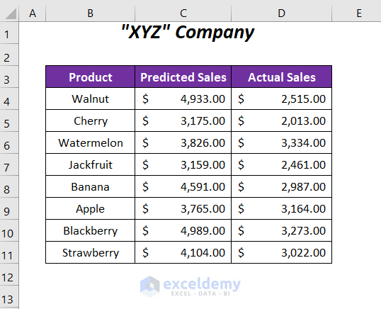
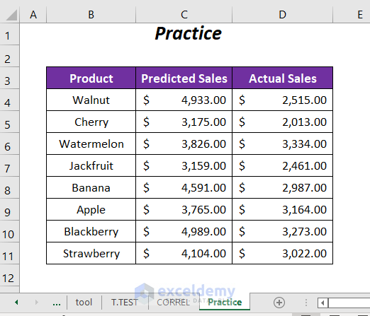
Dataset Overview

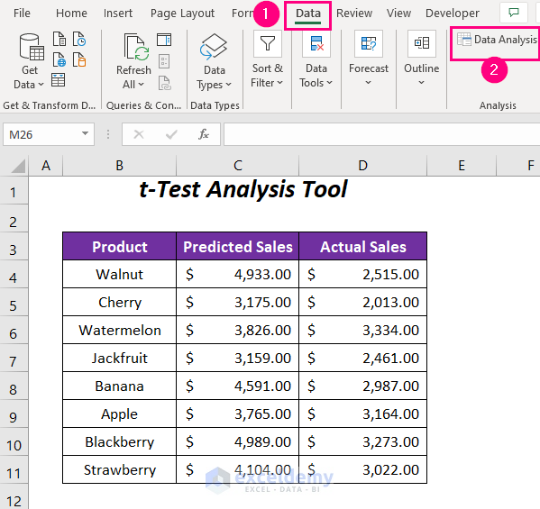
We have some predicted sales values and actual sales values of some of the products of a company.

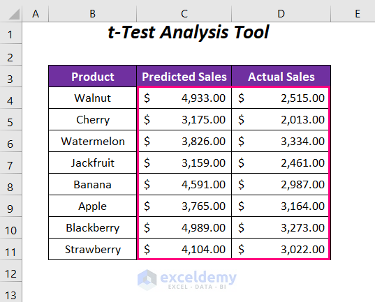
Method 1 – Using t-Test Analysis Tool

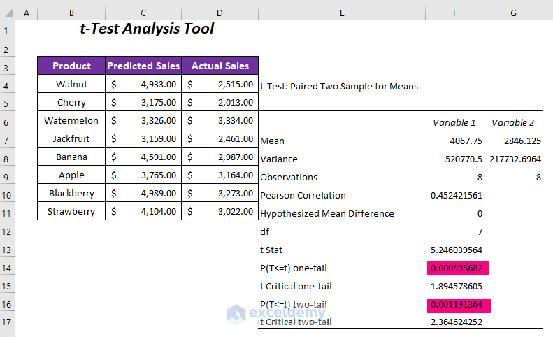
Here, we will use the Data Analysis Toolpak containing the t-Test analysis tool to determine the P-value for the two sets of sales data.

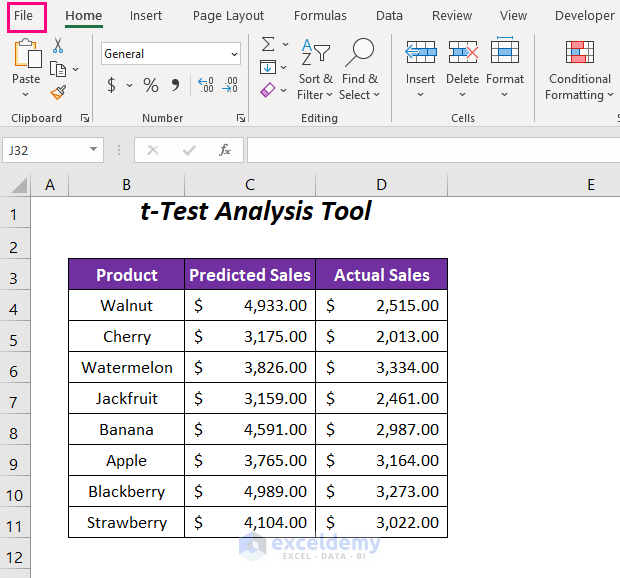
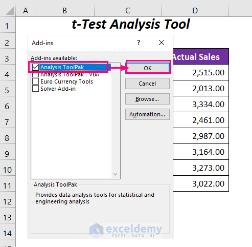
• Activate the Data Analysis ToolPak (if not already enabled):
  • Click on the File tab.

• • Select Options.

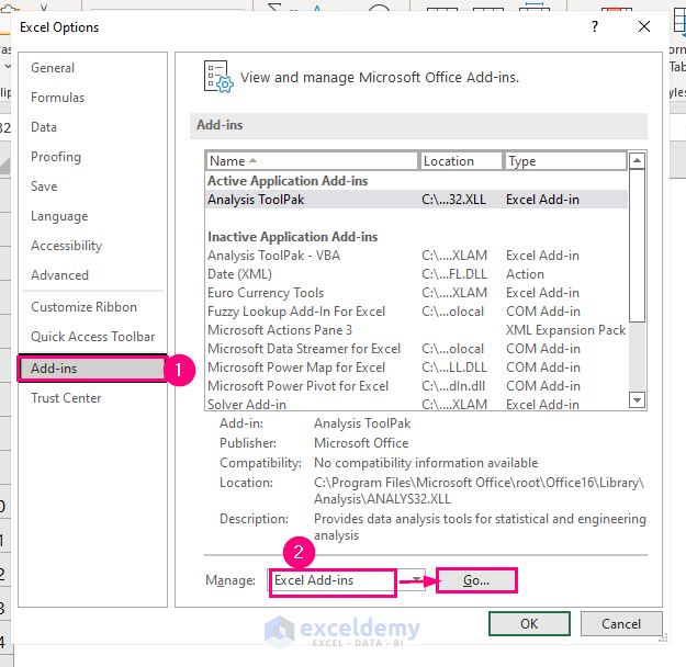
• • In the Excel Options dialog box, choose the Add-ins option on the left panel.
  • In the Manage box, select Excel Add-ins and click Go.

• • Check the Analysis ToolPak option and press OK.

• Access the Data Analysis Tool:
  • Go to the Data tab.
  • In the Analysis group, click on Data Analysis.

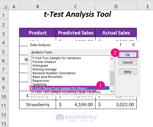
• Select the t-Test: Paired Two Sample for Means:
  • The Data Analysis wizard will appear.
  • Choose the option t-Test: Paired Two Sample for Means from the list of analysis tools.

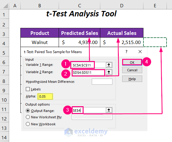
• Provide Input Ranges:
  • For Variable 1 Range, use the range $C$4:$C$11 (predicted sales values).
  • For Variable 2 Range, use the range $D$4:$D$11 (actual sales values).
  • Select an Output Range (e.g., $E$4).

• Set the Significance Level (Alpha):
  • You can change the value for Alpha (significance level) from the default 0.05 to 0.01 if needed.

• Calculate the P-Values:
  • Press OK.

• • You’ll obtain two P-values:
    • One-tail value: 0.00059568
    • Two-tail value: 0.0011913
  • Note that the one-tail P-value is half of the two-tail P-value. The former considers only one direction (increase or decrease), while the latter considers both directions.

• Interpretation:
  • For an Alpha value of 0.05, the P-values are less than 0.05, indicating that we reject the null hypothesis. The data is highly significant.

Method 2 – Using the T.TEST Function

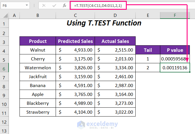
In this section, we will be using the T.TEST function to determine the P values for tails 1 and 2.

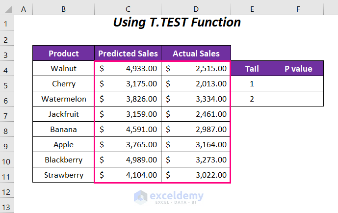
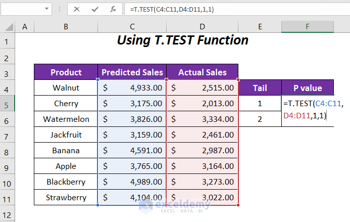
• Calculate P-Value for Tail 1 (One Direction):
  • In cell F5, enter the following formula:

Here,

• C4:C11: Predicted sales range
• D4:D11: Actual sales range
• 1: Tail value (one-tail test)
• Last 1: Paired type

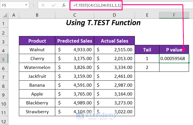
• Result for Tail 1:
  • The P-value for tail 1 is 0.00059568.

• Calculate P-Value for Tail 2 (Both Directions):
  • In cell F6, enter this formula:

Here,

• C4:C11: Predicted sales range
• D4:D11: Actual sales range
• 2: Tail value (two-tail test)
• Last 1: Paired type

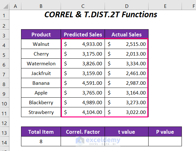
Method 3 – Using CORREL and T.DIST.2T Functions

In this method, we’ll determine the P-value for correlation using the CORREL and T.DIST.2T functions. Follow these steps:

• Create Columns:
  • Set up columns with the following headers: Total Item, Correl. Factor, t Value, and P value.
  • Enter the total number of items (which is 8) in the appropriate cell.

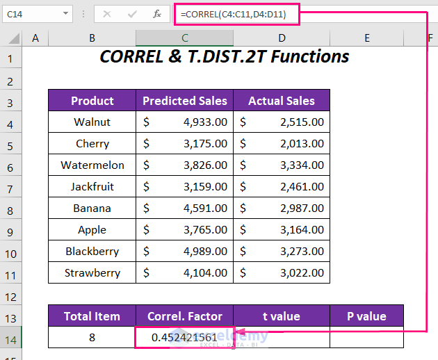
• Calculate the Correlation Factor (Correl.Factor):
  • In cell C14, enter the formula:

• • • Here, C4:C11 represents the range of predicted sales, and D4:D11 represents the range of actual sales.

• Determine the t Value:
  • In cell D14, enter the formula:

Here,

• C14 is the correlation factor, and B14 is the total number of products.
• Calculate intermediate values:
  • SQRT(B14-2) gives the square root of 6 (approximately 2.4494897).
  • C14*SQRT(B14-2) results in approximately 1.10820197.
  • 1-C14*C14 evaluates to approximately 0.79531473.
  • SQRT(1-C14*C14) returns approximately 0.891804199.
  • The final t value is approximately 1.242651665.

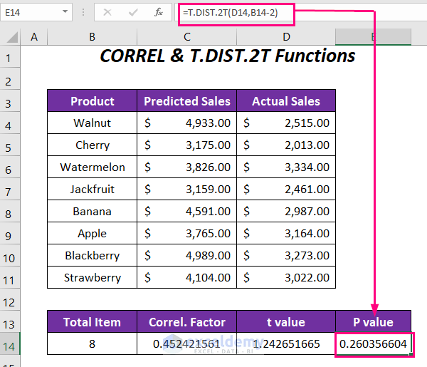
• Compute the P-Value for Correlation:
  • Use the following function:

Here,

• D14 represents the t value.
• B14-2 (or 8-2, which is 6) is the degrees of freedom.
• T.DIST.2T returns the P-value for correlation with a two-tailed distribution.

Read More: How to Do Multiple Regression Analysis in Excel

Things to Remember

• Alpha Values:
  • Commonly used significance levels are 0.05 and 0.01.
• Hypotheses:
  • The null hypothesis assumes no difference between the two data sets.
  • The alternative hypothesis considers a difference between the data sets.
• Interpretation:
  • P < 0.05: Highly significant data
  • P = 0.05: Significant data
  • P = 0.05-0.1: Marginally significant data
  • P > 0.1: Insignificant data

Practice Section

To practice we have provided a Practice section in a sheet named Practice.

Download Workbook

You can download the practice workbook from here:

Related Articles

• How to Do Simple Linear Regression in Excel
• How to Interpret Regression Results in Excel
• How to Interpret Multiple Regression Results in Excel
• How to Do Logistic Regression in Excel
• How to Plot Least Squares Regression Line in Excel
• How to Do Linear Regression in Excel
• Multiple Linear Regression on Excel Data Sets

<< Go Back to Regression Analysis in Excel | Excel for Statistics | Learn Excel