What Is Regression?
Regression analysis is often used in data analysis to determine the associations among multiple variables.
Simple linear regression is distinct from multiple linear regression in statistics. Using a linear function, simple linear regression analyzes the association between the variables and an independent variable. Multiple linear regression is when two or more factors are used to determine the variables. This article will focus on multiple linear regression on a data set.
How to perform Regression in Excel
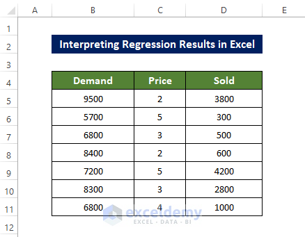
The dataset below will be used for analysis. The independent variable is: Price and Sold . The independent column is Demand .
Steps
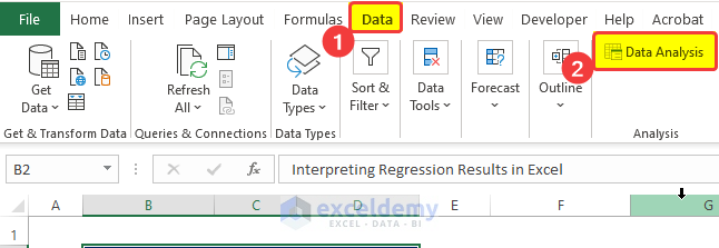
- Go to the Data tab and click on Data Analysis.
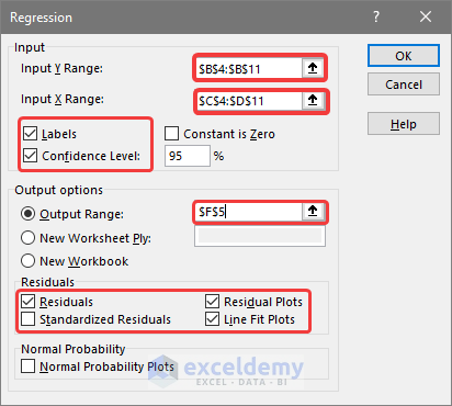
- In the new window; select the dependent variable and independent variable data range.
- Check Labels and Confidence.
- Click the output cell range box to select the output cell address.
- Check Residual to calculate the residuals.
- Check Residual Plots and Line Fit Plots.
- Click OK.
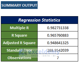
The primary output parameters of the analysis will be displayed.
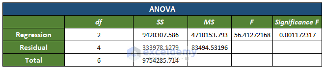
- Other parameters, for example Significance value, will also be displayed in the ANOVA (Analysis of Variance) table.
- df is the degree of freedom of the source of variance.
- SS is the sum of squares. (For better results, the Residual SS should be smaller than the Total SS).
- MS means square.
- F is the F-test for the null hypothesis.
- Significance F is the P-value of F.
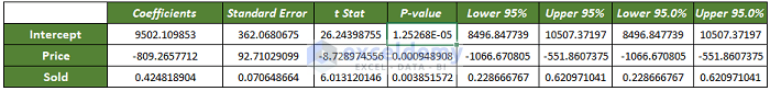
You will also see the variable’s coefficients, significance value, etc in a table.
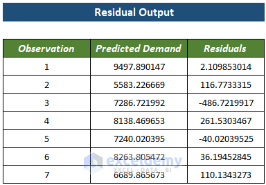
The coefficient table contains the residual value for each entry.
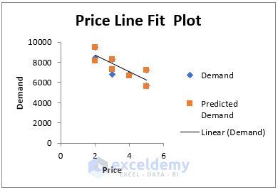
This is the Demand vs Price regression chart, with a trendline.
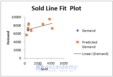
This is the Demand vs Sold regression chart with a trendline.
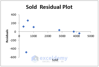
This chart shows the distribution of residuals for each entry of the Sold variable.
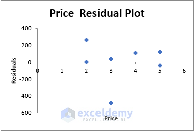
This chart shows the distribution of residuals for each entry of the Price variable.
How to Interpret Regression Results in Excel: Detailed Analysis
Multiple R-Squared Regression Value Analysis
The R-squared number indicates how closely the elements in dataset are related and how well the regression line matches the data. The multiple linear regression analysis will be used to determine the impact of two or more variables on the main factor. The range of this coefficient is from -1 to 1:
- 1 means a close positive relationship
- 0 means there are no relationships among variables.
- -1 means inverse or negative relationship among variables.
In the output results shown above, the multiple R-value of the given data sets is 0.7578(approx), which indicates strong relations between the variables.
R Squared
R squared value explains how the response of the dependent variables varies, according to the independent variable. Here, the value is 0.574(approx), which can be interpreted as a reasonable relationship between the variables.
Adjusted R-Squared
It is merely an alternative version of the R squared value. It shuffles the predictor variables, forecasting the response variable:
R^2 = 1 – [(1-R^2)*(n-1)/(n-k-1)]
Here, R^2: The R^2 value we got from the dataset.
n: the number of observations.
K: the number of predictor variables.
This value is significant in regression analysis between two predictor variables. If there is more than one predictor variable in the dataset, the R squared value will be inflated, which is highly undesirable. The adjusted R squared value adjusts this inflation and gives an accurate picture of the variables.
Standard Error
It is a goodness-of-fit metric that indicates the accuracy of your regression analysis; the lower the value, the more accurate is the regression analysis.
Standard Error is an empirical metric representing the average distance points deviate from the trendline. R2 represents the proportion of dependent variable variation. In this case, the value of Standard Error is 288.9 (approx), which means that our data points, on average, drop 288.9 from the trendline.
Observations
Indicate the number of observations or entries.
Determine Significant Variable
The Significance value indicates the trustworthiness (statistically sound) of the analysis. This value should be below 5%. But in this case, the significance value is 0.00117, which translates to 0.1% – well below the 5%. So the analysis is accurate.
P-value in Regression Analysis
The P-value represents the probability of the coefficient value being wrong: the association of the null hypothesis with the variables.
If your p-value < the Significance number, there is enough evidence to reject the null value hypothesis. This means there is a non-zero correlation between the variables.
If the p-value > Significance value, there will be insufficient evidence to dismiss the null hypothesis. There could be no correlation between the variables.
Here, the P-value of the variable Price =0.000948 < 0.00117 (significance value):
There is no null hypothesis, and there is enough evidence to declare a correlation between variables.
For the variable Sold, the (P-value) 0.0038515 < 0.0011723 (Significance value)
There could be a null hypothesis and there is not enough evidence to declare a non-zero correlation between variables.
Regression Equation
To determine the linear regression analysis in Excel, the trend line should also be linear. The general form is:
Y=mX+C.
Here, Y is the dependent variable.
And X is the independent variable: the effect of the change of variable x on variable Y will be determined.
C is the value of the Y-axis intersection of the line.
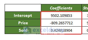 The value of the C intercept, here, is equal to 9502.109853
And the value of m for the two variables is -809.265 and 0.424818.
there’s a final equation for the two separate variables:
The first one is:
And the second is:
Coefficients
The coefficients, here, are m1=-809.2655 and m2=04248. And interceptor, C= 9502.12.
- The interceptor value indicates that the demand will be 9502 when the price is zero.
- And the values of m are the rate at which demand changes per unit of price change. The price coefficient value is -809.265, indicating that a per unit increase in price will drop the demand by roughly 809 units.
- For the second variable, Sold, the m value is 0.424. This shows that the change per unit sold item will result in a 0424-time unit increase of the product.
Residuals
The Residual is the difference between the original and the calculated entry from the regression line. Residuals indicate how distant the actual value is from the line. For example, the computed entry in the regression analysis for the first entry is 9497. And the first original value is 9500. The residual is around 2.109.
T-Statistics Value
T-statics value is the division of coefficient by the standard value. The higher the value, the more reliable are the coefficients.
It is used to calculate the P-value in linear regression.
The 95% Confidence Interval
Here the confidence of the variable was set as 95 at the beginning. It can change, though.
- Here, the coefficient value of the lower 95% is calculated as 8496.84. It means the upper 95% is calculated as 10507.37,
- While the main coefficient is about 9502.1, there is a high chance that the value is below 8496 for 95% of the cases and a 5% chance of being over 10507.37
Things to Remember
✎ The regression analysis method assesses the relationship among variables under examination. It doesn’t establish causation.
✎ Regression analysis hampers heavily by outliers. All kinds of outliers must be removed before analysis is done.
Download Practice Workbook
Download this practice workbook.
Related Article
- How to Interpret Linear Regression Results in Excel
- How to Interpret Multiple Regression Results in Excel
- How to Plot Least Squares Regression Line in Excel
- How to Do Logistic Regression in Excel
<< Go Back to Regression Analysis in Excel | Excel for Statistics | Learn Excel
Get FREE Advanced Excel Exercises with Solutions!
