How to Do Logistic Regression in Excel (with Quick Steps)

Regression analysis is a widely used statistical calculation. We often do this type of calculation according to our desire. In Excel, we can perform multiple types of regression analysis. In this article, we will demonstrate how to do logistic regression in Excel. If you are also interested to learn this analysis, download the practice workbook and follow us.

What Is Logistic Regression?

Logistic regression analysis is a statistical learning algorithm that uses to predict the value of a dependent variable based on some independent criteria. It helps a person to get the result from a large dataset based on his desired category. Logistic regression analysis mainly three types:

Binary Logistic Regression
Multinomial Logistic Regression
Ordinal Logistic Regression

Binary Logistic Regression: In the binary regression analysis model, we define a category by only two cases. Yes/No or Positive/Negative.

Multinomial Logistic Regression: Multinominal logistic analysis works with three or more classifications. If we have more than two classified sections to categorize our data, then we can use this regression analysis model.

Ordinal Logistic Regression: This regression analysis model works for more than two categories. However, in this model, we need a predetermined order to categorize them.

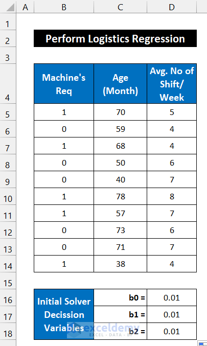
How to Do Logistic Regression in Excel: with Quick Steps

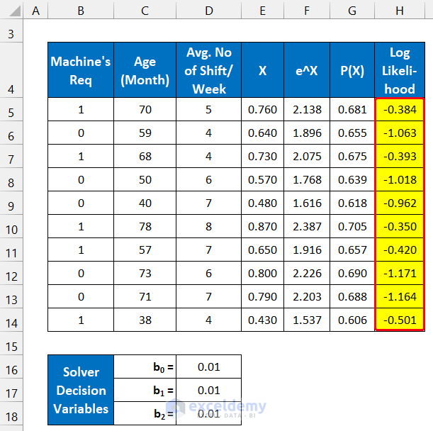
In this article, we will perform the binary logistical regression analysis. This type of analysis provides us with a prediction value of the desired variable. To perform the analysis, we consider a dataset of 10 machines from an industry. The machine’s availability can be positive or negative. The binary digits 1=positive, and 0=negative, and these values are shown in column B. The age of those machines is in column C and the average duty hours of them per week is in column D. So, our dataset is in the range of cells B5:D14. The values initial regression solver variable are in the range of cells C16:D18. 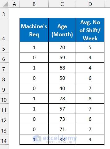The whole analysis procedure is explained below step by step:

Step 1: Input Your Dataset

In this step, we are going to import your dataset:

First of all, input your dataset accurately into Excel. For our analysis, we input the dataset in the range of cells B5:D14.

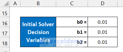
Then, input your Solver Decision Varibles’ We input them in the range of cells D16:D18.
We are assuming all the variables’ values as 0.01.

Step 2: Evaluate Logit Value

In this step, we are going to calculate the Logit value for our dataset. We define the Logit value as X in our calculation. The formula of Logit value is:

Here, b0, b1, and b2 are regression variables.

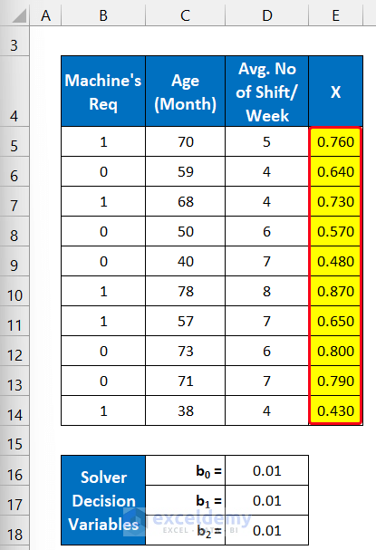
Write down the following formula in cell E5. Use the Absolute sign to freeze the cell value of variables. If you don’t know how to input the Absolute Cell Reference sign, you can input it in several ways.

=$D$16+$D$17*C5+$D$18*D5

Then, press the Enter key on your keyboard.

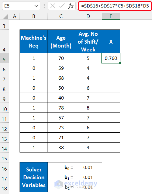
After that, double-click on the Fill Handle icon to copy the formula up to cell E14.

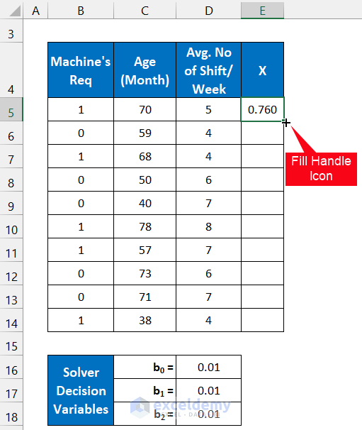
You will get all the values of X.

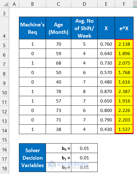
Step 3: Determine Exponential of Logit for Each Data

Here, we will calculate the exponential value of the logit value, For that, we are going to use the EXP function:

To determine the exponential value of X, write down the following formula in cell F5:

=EXP(E5)

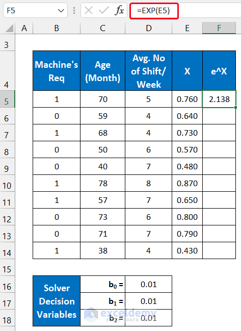
Similarly, double-click on the Fill Handle icon to copy the formula like the previous step. You will all the exponential values of X.

Step 4: Calculate Probability Value

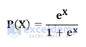
P(X) is the probability value for occurring the X event. The probability of event X can define as:

To calculate it, write down the following formula in cell G5.

=F5/(1+F5)

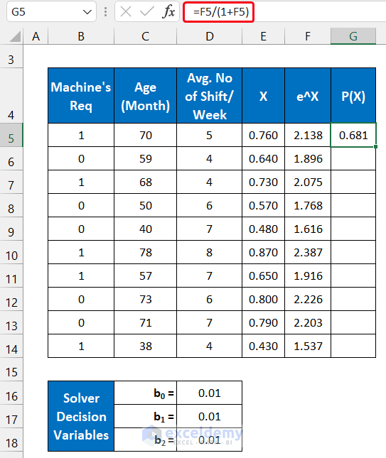
Press the Enter key.
Now, drag the Fill Handle icon up to G15 to get the value for all values.

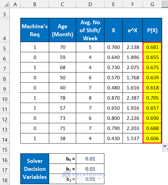
Step 5: Evaluate Sum of Log-Likelihood Value

In the following steps, we are going to evaluate the value of Log-Likelihood. After that we will use the SUM function to add all the data:

To calculate the Log-Likelihood value, we are going to use the LN function in our dataset. In cell H5, write done the following formula:

=(B5*LN(G5))+((1-B5)*LN(1-G5))

Now, press the Enter key on the keyboard.

Then, double-click on the Fill Handle icon to determine all log-likelihood values.

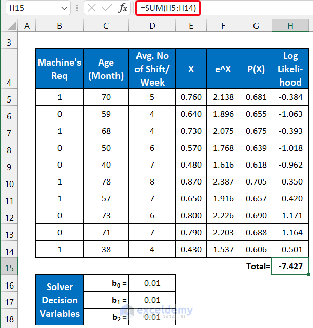
After that, in cell H15, write down the following formula to sum all the values.

=SUM(H5:H14)

🔍 Breakdown of the Formula

We are doing this breakdown for cell H5.

👉 LN(G5): This function returns -0.384.

👉 LN(1-G5): This function returns -1.144.

👉 (B5*LN(G5))+((1-B5)*LN(1-G5)): This function returns -0.384.

Step 6: Use Solver Analysis Tool for Final Analysis

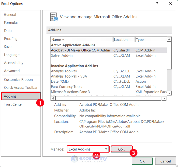
Now, we will conduct the final regression analysis. We will perform the analysis through the Solver command. If you don’t see it in the Data tab, you have to enable the Solver from the Excel Add-ins.

To enable it, select File > Options.

As a result, a dialog box called Excel Options will appear.
In this dialog box, select the Add-ins option.
Now, choose the Excel Add-ins option in the Manage section and click Go.

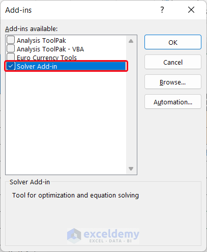
A small dialog box titled Add-ins will appear.
Then, check the Solver Add-in option and click OK.

After that, go to the Data tab, and you will find the Solver command in the Analysis group.

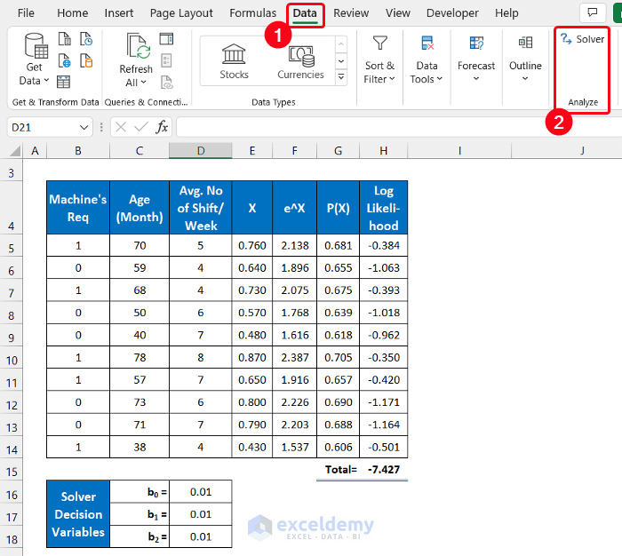
Now, click the Solver command.
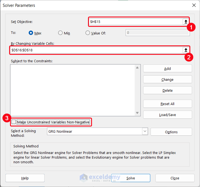
A new dialog box entitled Solver Parameters will appear.
In the Set Objective box, choose the cell $H$15 with your mouse. You can also write the cell reference on your keyboard. Make sure you use the Absolute Cell Reference sign here.
Next, in the By Changing Variable Cells option select the range of cells $D$16:$D$18.
Then, uncheck the Make Unconstrained Variables Non-Negative to get the negative values if it is already showing as checked.
Finally, click the Solve button.

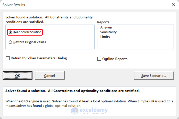
As a result, the Solver Result box will appear in front of you.
Now, choose the Keep Solver Solution This box will also show you whether your regression analysis converged or diverged.
Click OK to close the box.

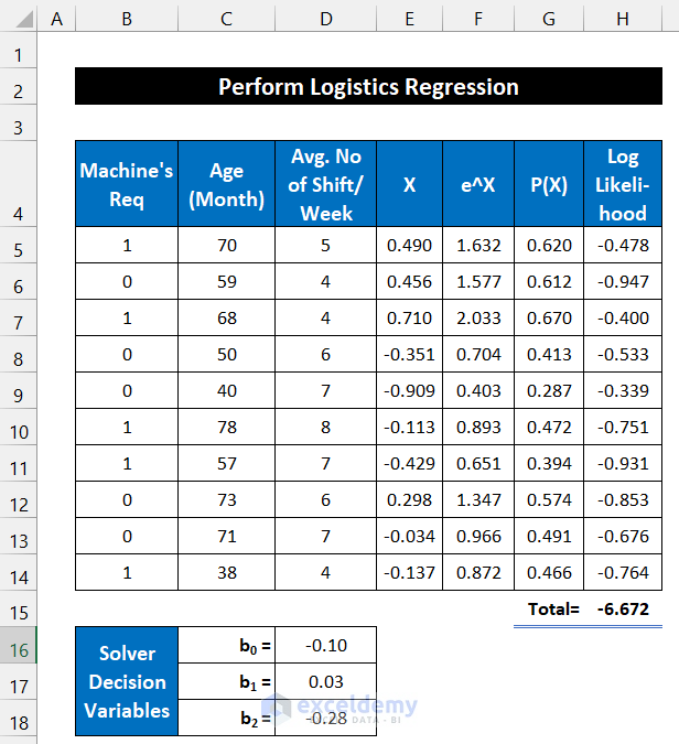
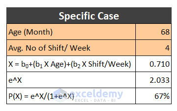
At last, you will see the values of the variable in the range of cells D16:D18 is changed. Besides it, you will also see the values of columns E, F, G, and H are also showing differences from the previous steps.

🔍 Illustration of Binary Regression Analysis Result

After the completion of the binary logistic regression analysis in Excel, you will see that our assumed regression variable value is substituted with the new analysis value and these values are the correct regression variable value of our dataset. We can consider the result of any specific data, like the machine which has an age of 68 months and 4 avg. no shift per week. The value of P(X) is 0.67. It illustrates to us that if we look for the machine in working condition the possibility of that event is about 67%.

We can also show it separately, using the final values of the regression variable.

Thus, we can say that our working procedure worked successfully and we are able to do binary logistic regression analysis.

Download Practice Workbook

Download this practice workbook for practice while you are reading this article.

Logistic Regression.xlsx

Conclusion

That’s the end of this article. I hope that this article will be helpful for you and you will be able to do logistic regression in Excel. Please share any further queries or recommendations with us in the comments section below. Keep learning new methods and keep growing!

<< Go Back to Regression Analysis in Excel | Excel for Statistics | Learn Excel

Get FREE Advanced Excel Exercises with Solutions!

6 Comments

Ella Dec 9, 2022 at 4:30 AM

Hi! How do you assume what b0, b1 and b2 are? Are there always 3 or is it one for the dependent+1 for each indicator you are testing?
- Reply
  Afia Dec 12, 2022 at 2:39 PM
  
  Dear Ella,
  Thank you for your comment. I will try to provide a proper answer to your question.
  
  The first answer is, to set the value for b0, b1, and b2, you can assume any values. Then, you can optimize the assumed values.
  
  The answer to the second question is, since we have 2 independent and one dependent variable, we took 3 initial problem-solver variables. One for the dependent variable, and then for each independent variable, we took 1 additional problem solver variable.
  
  I hope this will help you.
  
  Regard,
  Afia Aziz Kona
Seun Olaleye Mar 2, 2023 at 8:12 PM

Thank you for this post. Very instructive.
What if I have more than 2 independent variables (5 to be specific), how do i use the Log-Likelihood formula, :
=(B5*LN(G5))+((1-B5)*LN(1-G5))
Does it remain as is or does it change based on the number of independent variables?
- Reply
  Shahriar Abrar Rafid Mar 9, 2023 at 5:27 PM
  
  Hello SEUN OLALEYE,
  Hope you are doing all well. Let’s get into your query first.
  In this case, the Log-Likelihood formula doesn’t rely on the number of independent variables. In the case of 5 independent variables, the formula would be the same. The change will happen in the formula of the Logit value (X).
  X = b0 + (b1 * ind var 1) + (b2 * ind var 2) + (b3 * ind var 3) + (b4 * ind var 4) + (b5 * ind var 5)
  The only change will happen here. All the remaining formulas will be the same.
  For a better understanding, please go through the entire article again. Happy Excelling.
  Regards,
  SHAHRIAR ABRAR RAFID
  Team ExcelDemy
Mike M Mar 24, 2023 at 10:18 PM

Hello, Im having an issue. Sometimes after pressing the Solve button, it comes back with an error stating “one of the cells in the worksheet became an error value when Solver tried certain values for the Variable Cells”. When I go back to the worksheet, there is a #NUM! error in one or 2 cells in the Exponential Value column.

Any ideas as to why this is happening? Any help would be greatly appreciated.
- Reply
  Mohammad Shah Miran Mar 27, 2023 at 11:18 AM
  
  Thanks, MIKE M for your question. The problem you are stating indicates that the Solver could not find a solution that satisfied the optimization constraints you specified. This can happen for several reasons, including Incorrect input data, Incorrect model specification, Insufficient or incorrect constraints, Numerical instability, etc. Try to rectify those issues or if you need a more specific solution to your problem, it would be convenient if you provide your dataset. Thanks for being with ExcelDemy.
  
  Regards
  Mohammad Shah Miran
  Team ExcelDemy