How to Perform Multiple Linear Regression in Excel (2 Methods)

What Is Multiple Linear Regression?

Multiple linear regression (or simply multiple regression) is a statistical technique that predicts the outcome of a dependent variable based on several independent variables. It extends the concept of simple linear regression, which involves only one independent variable.

Suppose we have two independent variables, denoted as X1 and X2, affecting the value of a dependent variable Y. The equation for multiple linear regression is:

Here,

• α stands for the Intercept (constant).
• α₁ and α₂ represent the change in Y due to the changes in X₁ and X₂ respectively.
• ϵ signifies the residual or error.

Multiple linear regression assumes a linear relationship between the dependent variable (Y) and the independent variables (X1 and X2). However, it also considers that the relationship between the independent variables may be statistically insignificant.

This technique finds extensive use in financial inference and econometrics.

Dataset Overview

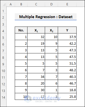
Consider the following dataset, which contains information about 10 houses (numbered 1 to 10). The variables are as follows:

• X₁ indicates the age of the houses.
• X₂ denotes the number of grocery stores near each of them.
• Y prices per unit area of the houses (Y is the dependent variable).

Method 1 – Performing Multiple Regression in Excel

To perform multiple linear regression in Excel, follow these three steps:

• Enable the Analysis ToolPak:

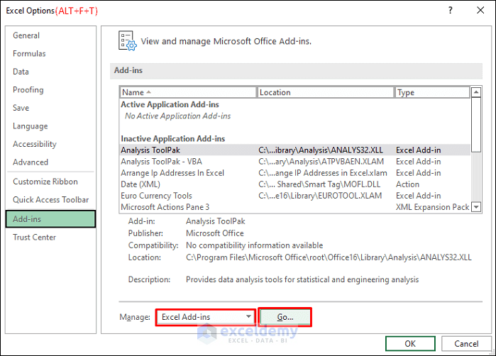
• • Press ALT+F+T to open Excel Options.
  • Go to the Add-ins tab and select Excel Add-ins.

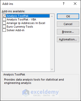
• • Check the “Analysis ToolPak” checkbox and click OK.
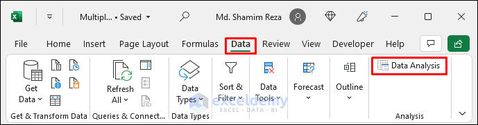
  • You can now access the Data Analysis feature from the Data tab.

• Perform the Regression Analysis:
  • Select Data > Data Analysis.

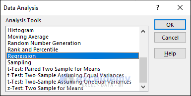
• • In the Data Analysis dialog box, scroll through the Analysis Tools and choose Regression. Click OK.

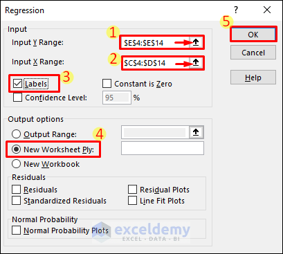
• • Specify the Y range (including header cells) as $E$4:$E$14 and the X range as $C$4:$D$14.
  • Check the “Labels” checkbox and choose any desired output options. Click OK.

You will see the analysis result in detail as shown in the following picture.

• Interpret the Results:
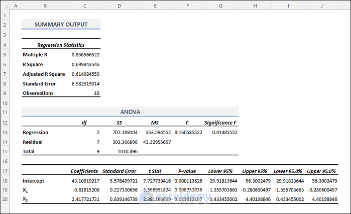
  • The analysis result will display detailed information, including the Regression Statistics table, ANOVA table, and Regression Coefficients table.
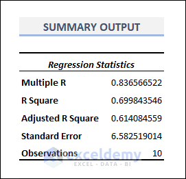
  • Pay particular attention to the R-squared value (explained variance) and the standard error (estimated deviation for the residual).

• • R Square = 0.6998 means 69.98% of the variables can be explained by the regressors or the independent variables.
  • The Standard Error signifies the estimated standard deviation for the residual or error.

Interpret the ANOVA Table

• Now, the Analysis of Variance (ANOVA) table is given below.

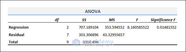
• Here, df stands for the degree of freedom and SS signifies the sum of squares of variances.
• The Significance F column has a P-Value of 0148 which is less than 5%. So, we can reject the Null Hypothesis. It concludes that the impact of the independent variables on the dependent variable is statistically significant.

Interpret the Coefficients Table

• The table below containing the coefficients and other outputs is of the most importance.

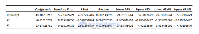
• We get the following coefficients from the table above. α₀ = 43.11, α₁ = – 0.82, α₂ = 2.42, and ϵ = 6.58. Therefore, the equation becomes:

Method 2 -Multiple Linear Regression with the LINEST Function

Alternatively, you can utilize the LINEST function in Excel to obtain regression results. Follow these steps:

• Enter the Formula:
  • In cell H5, enter the following formula:

• • • This formula calculates the desired results.

• Handling Errors:
  • Excel may display errors in some cells. To handle this, nest the LINEST function inside the IFERROR function:

How Does the Formula Work?

Objectives:

The LINEST function provides statistics describing a linear trend that matches known data points by fitting a straight line using the least-squares method.

Syntax:

Arguments:

• known_ys: Required. The dependent variable i.e. the Y range.
• [known_xs]: Optional. The independent variables i.e. the X₁ and X₂ ranges.
• [const]: Optional. True – constants are calculated normally. False – constants are set equal to zero.
• [stats]: Optional. True – returns the additional regression statistics. False – do not return additional regression statistics.

Read More: How to Do Linear Regression in Excel

Things to Remember

• Excel has a limit on the number of regressors (typically around 16). Ensure you don’t use more independent variables than allowed.
• Keep the regressors (independent variables) in adjoining columns.
• Excel assumes that errors are independent with constant variance (homoskedastic) and does not provide alternative assumptions.

Download Practice Workbook

You can download the practice workbook from here:

Related Articles

• How to Interpret Multiple Regression Results in Excel
• How to Interpret Regression Results in Excel
• How to Do Logistic Regression in Excel
• How to Calculate P Value in Linear Regression in Excel
• How to Interpret Linear Regression Results in Excel
• How to Plot Least Squares Regression Line in Excel

<< Go Back to Regression Analysis in Excel | Excel for Statistics | Learn Excel