In this article, we will show 10 practical examples of how to concatenate names in Excel.
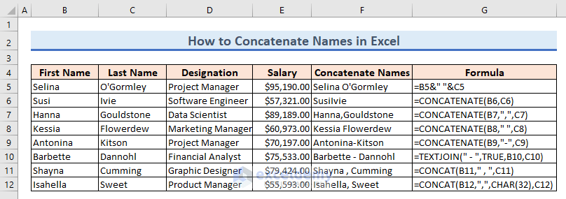
Suppose we have a dataset that contains the salary statements of several employees. We can use the Ampersand symbol, Flash Fill feature, CONCATENATE, CONCAT, TEXTJOIN, TEXT and CHAR functions, VBA code, and Power Query Editor to concatenate names in Excel.
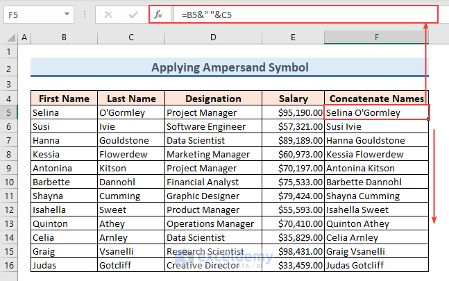
Method 1 – Using the Ampersand Symbol
The Ampersand symbol (&) can join or concatenate two or more cell values containing text.
Steps:
- Enter the following formula in cell F5 and press Enter:
=C5&" "&D5- Drag the AutoFill handle down to copy this formula to the cells below.
Notes:
Combine names with commas as follows:
=C5&" , "&D5Read More: How to Concatenate Date and Time in Excel
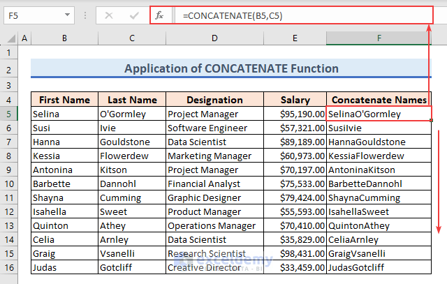
Method 2 – Using the CONCATENATE Function
The CONCATENATE function joins the values of two cells with or without spaces, delimiters or cell values with text, and can use the array formula.
2.1 – Concatenate First and Last Names Without Spaces
Let’s concatenate First and Last Names without spaces.
Steps:
- In cell F5, enter the following formula:
=CONCATENATE(B5,C5)- Press Enter and drag the AutoFill Handle to copy this formula to the cells below:
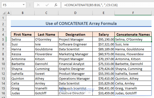
2.2 – Using an Array Formula
Let’s concatenate the First Name and Last Name of each employee into one single cell using an Array Formula.
Steps:
- Insert the following Array Formula in cell F5:
=CONCATENATE(B5:B16,", ",C5:C16)- Press Enter (or Ctrl + Shift + Enter if you are not an Excel 365).
Formula Breakdown:
If we break the Array Formula, we get 12 single formulas like this:
- CONCATENATE(B5,”, “,C5)
- CONCATENATE(B6,”, “,C6)
- CONCATENATE(B7,”, “,C7)
…
…
…
- CONCATENATE(B16,”, “,C16)
CONCATENATE(B5,”, “,C5) joins the First Name in cell B5, a comma with a space, and then the Last Name in cell C5. Same for the rest of the cells.
2.3 Using a Delimiter
Now we will join Names with delimiters like commas, spaces, different punctuation marks or other characters such as a slash or hyphen.
Steps:
- To join multiple cells with commas: enter the following formula in cell C19:
=CONCATENATE(B5,",",C5)- To join multiple cells with spaces: enter the following formula in cell C20:
=CONCATENATE(B6," ",C6)- To join multiple cells with hyphens: enter the following formula in cell C21:
=CONCATENATE(B7,"-",C7)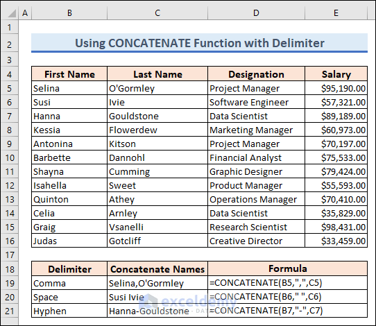
Read More: How to Combine Names in Excel with Space
Method 3 – Using the Flash Fill Feature
The Flash Fill feature of Excel can recognize a sequence in a provided range and fill the lower cells using the same pattern.
Steps:
- Enter the First Name and Last Name manually in cell F5.
- Go to Home → Editing → Fill → Flash Fill.
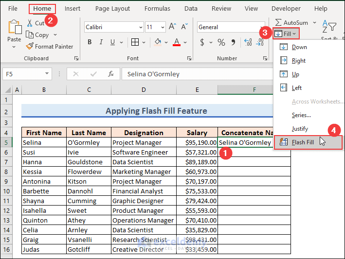
- Autofill the names of the rest of the cells into column F:

Notes:
You can also concatenate names using keyboard shortcuts. Enter the first and last names and press Ctrl + E.
Read More: How to Combine Name and Date in Excel
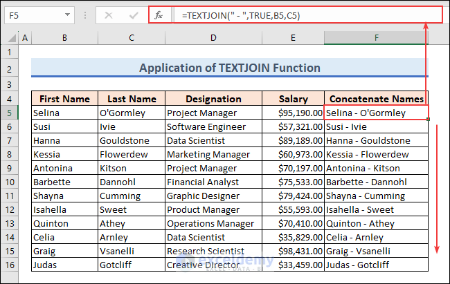
Method 4 – Using the TEXTJOIN Function
The TEXTJOIN function allows us to add multiple texts or values inside a single cell using a delimiter. Let’s apply it to our First and Last Names with a hyphen as a delimiter.
Steps:
- Enter the following formula in cell E5:
=TEXTJOIN(", ",TRUE,B5,C5)- Use the AutoFill handle to copy the formula to the rest of the cells in column E:
Read More: How to Concatenate Date/Day, Month, and Year in Excel
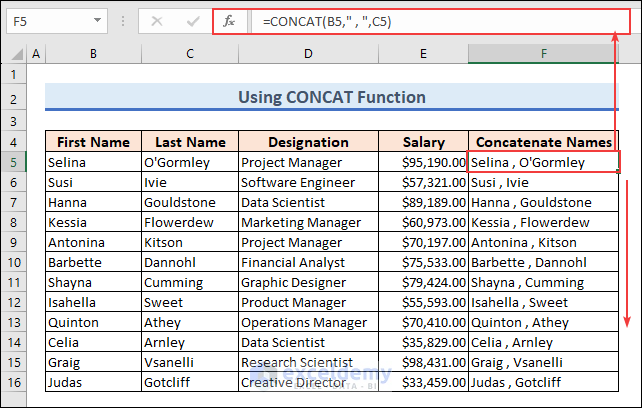
Method 5 – Using the CONCAT Function
The CONCAT function works similarly to the CONCATENATE function.
Steps:
- In cell F5, enter the below formula:
=CONCAT(C5," , ",D5)- Press Enter and use Fill Handle to apply this formula to the rest of the cells in column F:
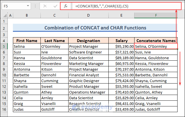
Method 6 – Combining the CHAR and CONCAT Functions
The CHAR function is useful to insert delimiters inside a join formula. In this example, we will combine CHAR and CONCAT functions to concatenate names.
Steps:
- In cell E5 enter the following formula and press Enter:
=CONCAT(C5,",",CHAR(32),D5)- Copy this formula down to cell E20 by dragging the AutoFill Handle.
Method 7 – Using a Line Break
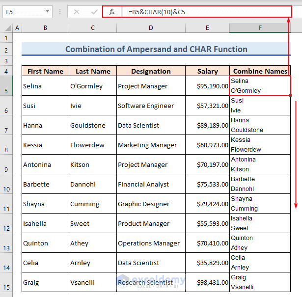
In this example, we will concatenate the First Names, Last Names, Designation, and Salary of the employees with a Line break using the Ampersand (&) symbol or CONCATENATE function along with the CHAR function. The CHAR(10) function in Excel returns the character represented by the ASCII value 10, which is a line break or newline character. This function is commonly used to insert line breaks or start a new line within a cell.
7.1 Using the Ampersand Symbol and CHAR Function
Steps:
- In cell F5, enter the following formula:
=B5&CHAR(10)&C5- Press Enter and then use the AutoFill handle to copy the formula to the rest of the cells in column F.
Now we will concatenate not only names but also other parameters like designations and salary.
- Enter the following formula in cell G5 and press Enter, then AutoFill the formula to the rest of the cells in column G:
=B5& " "&C5&CHAR(10)& D5 & "- " & E5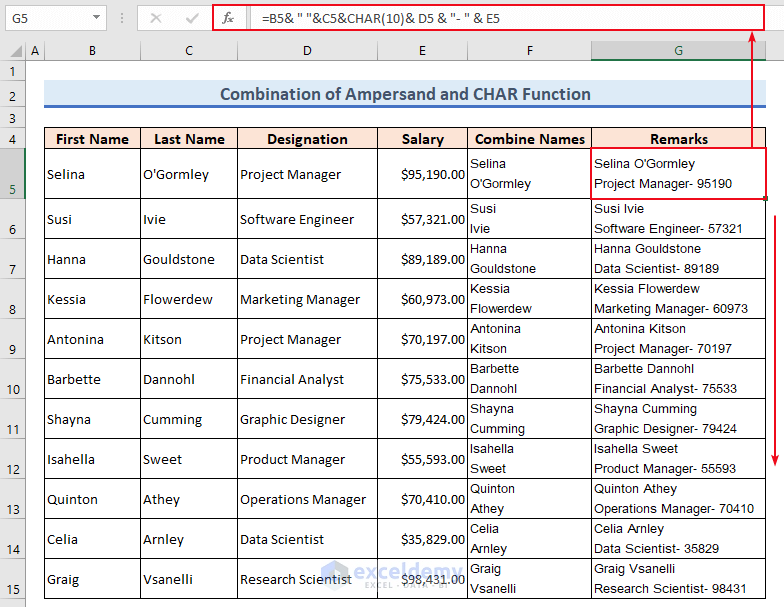
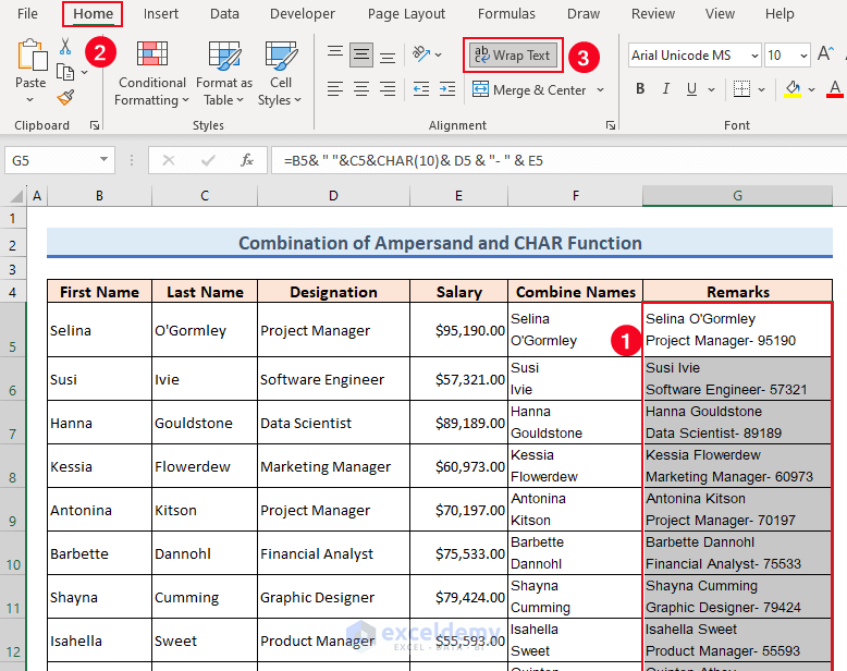
Notes:
Excel occasionally fails to insert a line break when we use the CHAR(10) function. To solve this issue, use the Wrap Text command, which is in the Alignment group under the Home tab.
7.2 – Using the CONCATENATE and CHAR Functions
Steps:
- In cell F5, enter the following formula:
=CONCATENATE(B5& " "&C5&CHAR(10)& D5 & "- " & E5)- Press Enter and use the AutoFill handle to copy the formula to the rest of the cells in column F.
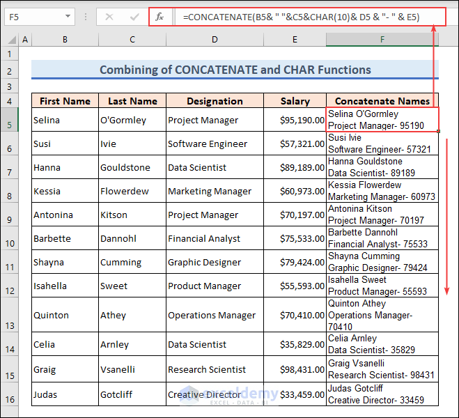
Formula Breakdown:
=CONCATENATE(B5& ” “&C5&CHAR(10)& D5 & “- ” & E5)
- The CONCATENATE function combines the value of cells B5, C5, D5, and E5.
- The CHAR(10) function breaks the line between the value of cells C5 and D5.
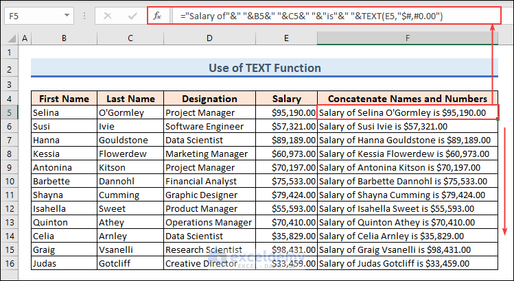
Method 8 – Using the TEXT Function to Concatenate Names and Number Values with Formatting
Now we will join the Name and Salary of the employees, i.e. joining a text value with a number.
Steps:
- Enter the following formula in cell F5, and press Enter:
="Salary of"&" "&B5&" "&C5&" "&"is"&" "&TEXT(E5,"$#,#0.00")- Drag the AutoFill handle to copy the formula down to cell F16.
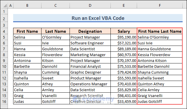
Method 9 – Running a VBA Code
Using a VBA Macro, we will combine the First Name and Last Name columns.
Steps:
- Press ALT + F11 to bring up the Visual Basic Application (or select the Visual Basic feature from the Developer tab).
- Select Insert >> Module.
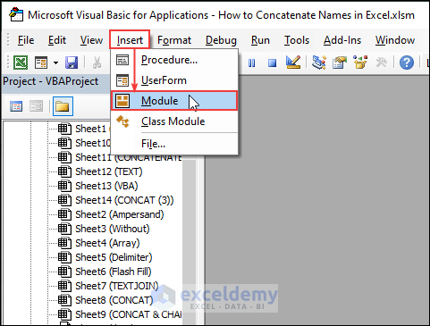
- Enter the following code in the Module window that opens, and click the Run button or press the F5 key to run the code:
Sub Concatenate_Names()
	Dim lastRow As Long
	Dim i As Long
	'Find the last row of data in column B
	lastRow = Cells(Rows.Count, "B").End(xlUp).Row
	'Loop through each row and concatenate the values from columns B, and C
	For i = 1 To lastRow
    	Cells(i, "F").Value = Cells(i, "B").Value & " " & Cells(i, "C").Value
	Next i
End Sub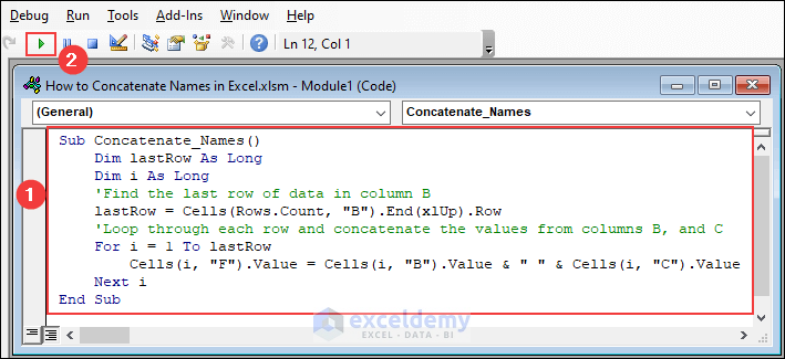
- The names are concatenated, along with the header of the columns.
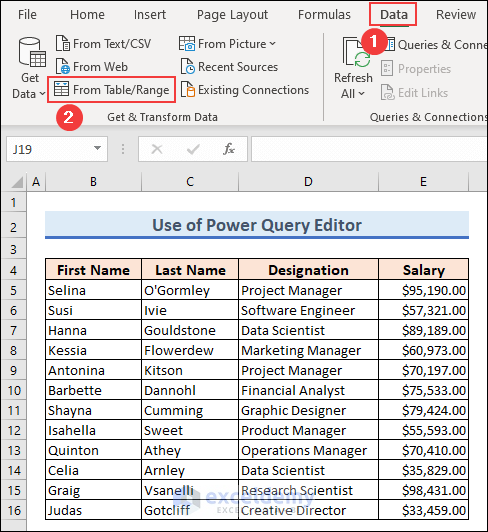
Method 10 – Using Power Query Editor
Steps:
- Go to the Data tab.
- Select From Table/Range from the Get & Transform Data group.
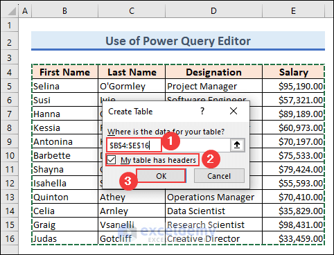
- In the Create Table window that opens, select the table location and check the My table has headers option.
- Click OK.
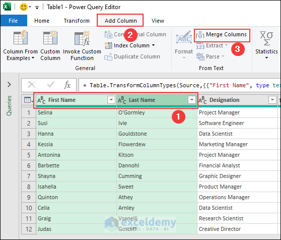
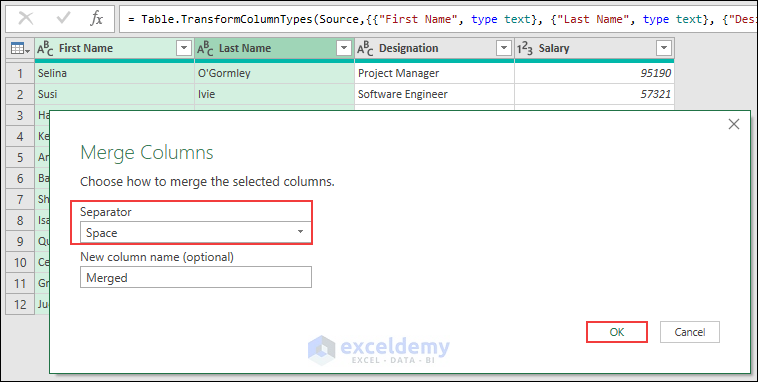
- In the Power Query Editor window that opens, select the three columns using Ctrl + Left Click.
- Go to the Add Column tab.
- Click on the Merge Columns feature from the From Text group.
- In the Merge Columns window, select Comma from the separator drop-down list and give the new column a name.
- Click OK.
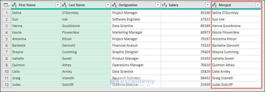
The result is as follows:
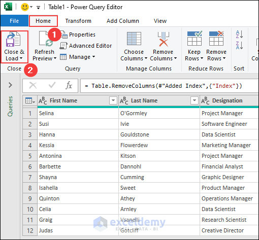
- Go to the Home tab and click on Close & Load.
- A new column is created containing the joined text as desired

Read More: Excel VBA: Combine Date and Time
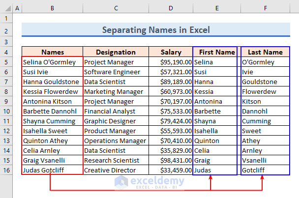
How to Separate Names in Excel
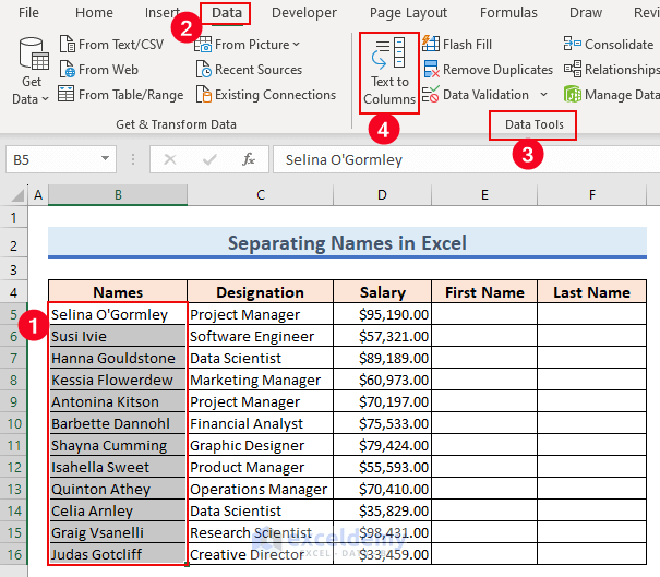
Let’s separate the First Name and Last Name from the Names column using the Text to Columns feature.
Steps:
- Select the data range of names, for example B5:B16 from our dataset.
- Go to the Data tab.
- Select the Text to Columns feature from the Data Tools group.
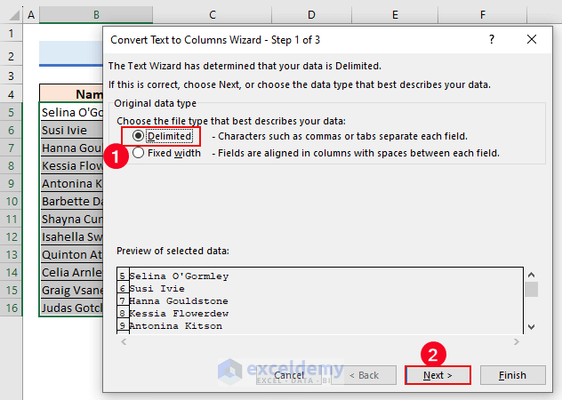
The Convert Text to Columns Wizard – Step 1 of 3 dialog box pops up.
- Check the Delimiter option and click the Next button.
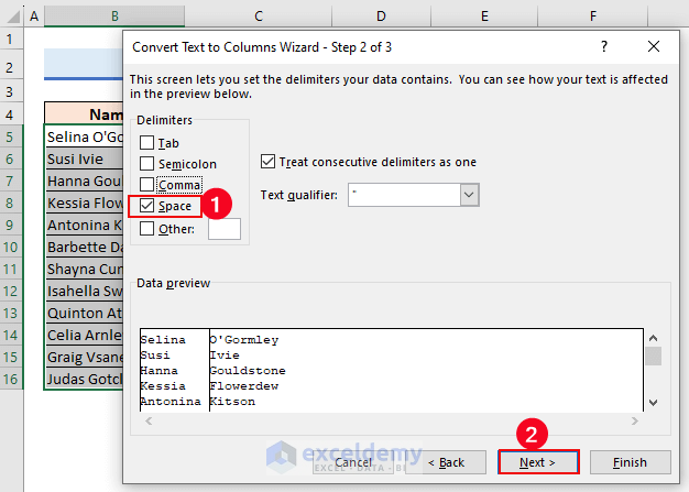
- Check the Space option from the Delimiters and click Next.
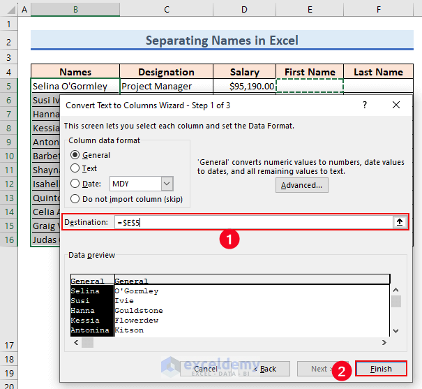
- Enter =$E$5 in the Destination box.
- Click the Finish button.
- A warning message is displayed.
- Click OK.
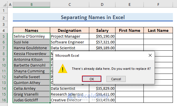
The text is separated into columns as desired.
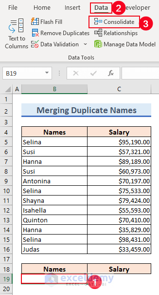
How to Merge Duplicate Names in Excel
If you have duplicate names in a single column and want to merge them to find their total, then the following method will be helpful.
Steps:
- Make new fields for storing the results after merging.
- Go to the Data tab.
- Choose Consolidate from the Data Tools group.
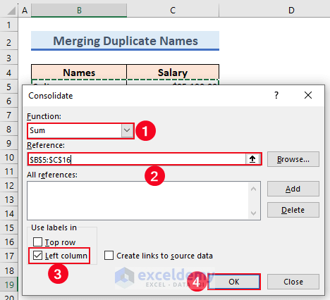
The Consolidate dialog box will appear.
- Select Sum under the Function dropdown list.
- Provide the cell range for consolidating.
- Check the Left column option from the Use labels in header.
- Click OK.
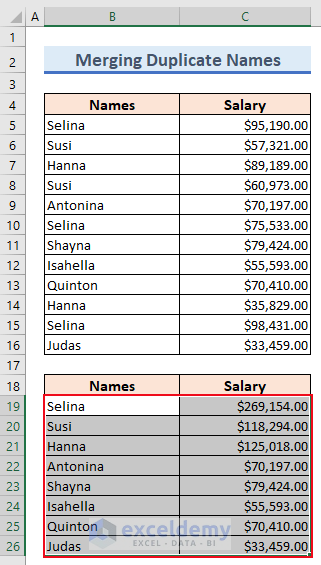
The cells that contain duplicate names are merged.
Read More: How to Combine Two Formulas in Excel
Things to Remember
- While writing syntax for functions and the ampersand, take care to insert proper space and quotation marks.
- Use the Power Query on your data range after converting it into a table. This will make the combination process easier.
Frequently Asked Questions
1. Can I concatenate names with a title or salutation included?
Yes, as a text string within the formula. For example, =CONCATENATE(“Mr. “, A1, ” “, B1) or =”Mr. ” & A1 & ” ” & B1.
2. Can I concatenate names with a specific capitalization format?
Yes, by using functions like UPPER, LOWER, or PROPER. For example, to capitalize only the first letter of each name component, use =PROPER(A1) & ” ” & PROPER(B1).
3. How can I concatenate multiple names with a comma separator?
Use the CONCATENATE function or the ampersand (&) operator. For example, =CONCATENATE(A1, “, “, B1) or =A1 & “, ” & B1.
Download Practice Workbook
Related Articles
<< Go Back to Concatenate Excel | Learn Excel
Get FREE Advanced Excel Exercises with Solutions!
