You may sometimes need to flip or reverse the order of columns vertically or horizontally while working with datasets in Excel. This can be necessary to take a peak at the end or to look at it from different perspectives and many other things. This article will focus on how to reverse the order of columns vertically in Excel.
How to Reverse Order of Columns Vertically in Excel: 3 Easy Ways
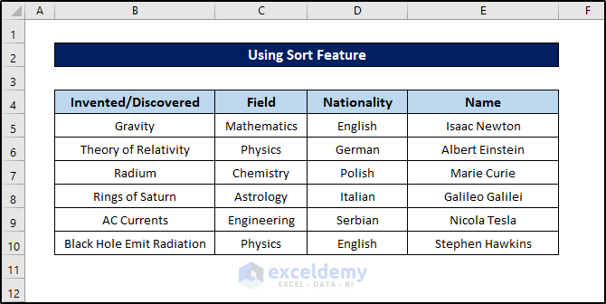
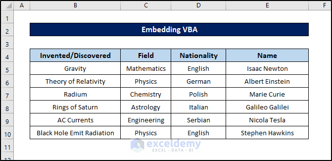
For all methods, we are going to use the following dataset.
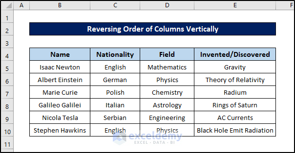
The dataset contains four columns- Name, Nationality, Field, and Invented/ Discovered. We are going to reverse the order of these columns from this to Invented/Discovered, Field, Nationality, and Name within Excel. We can achieve that by using the sort feature of Microsoft Excel, functions, and using VBA. Each is demonstrated in its section. Follow along to see how each works or find the one you need from the table above.
1. Using Sort Feature
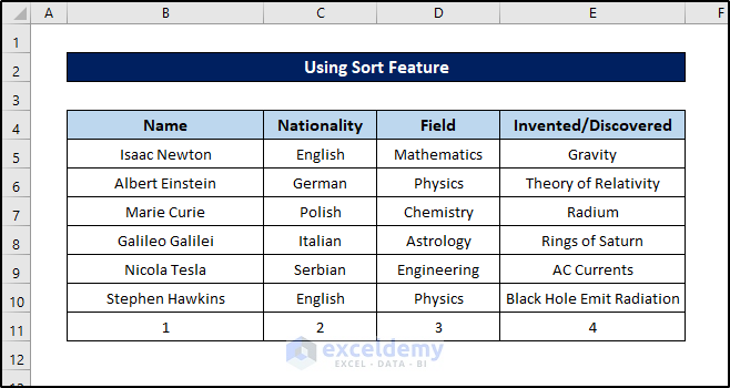
The first method we are going to use to reverse the order of columns vertically is to use the sort feature of Microsoft Excel. This feature usually sorts data by alphabetic or numeric ascending or descending order. So we cannot directly reverse the order of columns vertically(or even horizontally) in Excel. But we can work around this. All we need is to associate a helper row that assigns a number to each of the columns and then rearrange them using this feature.
Follow these steps to see the detailed guide.
Steps:
- First of all add numbers below each column. Here, our dataset ended at the 10th row of the spreadsheet. So we are adding numbers in the 11th row.
- Now select the whole dataset.

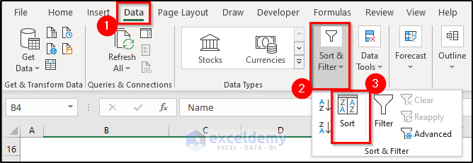
- After that, go to the Data tab on your ribbon.
- Then select Sort from the Sort & Filter group.
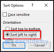
- As a result, the Sort box will open up. Now select Options here.

- Next, select Sort left to right in the Sort Options box and then click on OK.
- After that, going back to the Sort box, select Row 11 in the Sort by field.
- Then select Cell Values in the Sort On field.
- Next, select Largest to Smallest in the Order field.

- After clicking on OK the dataset will look something like this.

- Finally, remove the final row which we added in the first step.
This is one way you can reverse the order of Excel columns vertically.
Read More: How to Reverse Column Order in Excel
2. Using SORTBY and COLUMN Functions
In the next method, we are going to achieve the same result from the same dataset. But this time we are going to use a formula consisting of the SORTBY and COLUMN functions.
The SORTBY function can take several arguments. The primary arguments are the array it is sorting and the array it is using as the reference to sort. It can also take some sorting orders as optional arguments.
The COLUMN function can take a cell or an array as an argument and returns the column number of the cell (or an array in case of array input).
Follow these steps to see how we can use the combination of these to reverse the order of Excel columns vertically.
Steps:
- First, select the cell where you want your reversed dataset to start. We are selecting cell B12 for this.
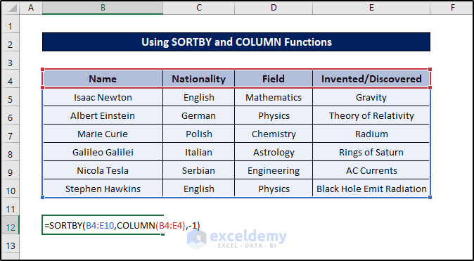
- Now write down the following formula in the cell.
=SORTBY(B4:E10,COLUMN(B4:E4),-1)
🔎 Breakdown of the Formula
👉 COLUMN(B4:E4) takes the range B4:E4 as an argument and returns all the column numbers within it as an array. The range takes up from the second to the fifth row of the spreadsheet. So it returns the array {2,3,4,5}
👉 SORTBY(B4:E10,COLUMN(B4:E4),-1) sorts the range B4:E10. It takes the previously mentioned array as the sort index. -1 (the third argument) indicates it will sort by descending order.
- After that, press Enter on your keyboard. This will result in an array like this.

- Finally, make some modifications to it.
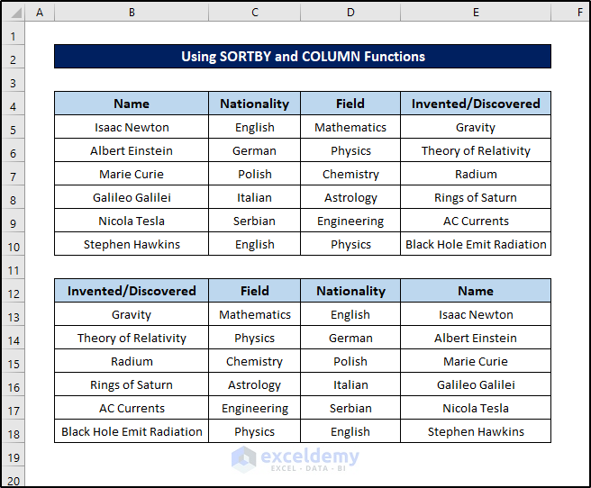
This is another way you can reverse the order of columns vertically in Excel.
3. Embedding VBA Code
The third method we are going to use is to reverse the order of the Excel column vertically to achieve the same result. The Visual Basic for Applications (VBA) is an event-driven programming language from Microsoft. It can be used to perform various tasks, sometimes otherwise impossible, in Microsoft Office applications. But to use VBA, you first need to enable the Developer tab. Click here to see how you can show the Developer tab on your ribbon.
Once you have that on your ribbon, follow these simple steps to reverse the order of columns vertically in Excel.
Steps:
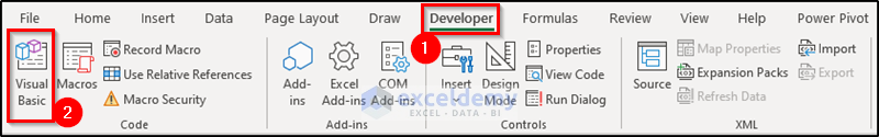
- First of all, go to the Developer tab.
- Then select Visual Basic from the Code group.
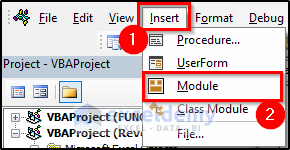
- As a result, the VBA window will open up. Now select the Insert tab in the window.
- Then select Module from the drop-down.
- Thus a new module will open up. Now select the newly created module and enter the following code in it.
Sub Reverse_Column_Order()
 Dim top_var As Variant
 Dim bot_var As Variant
 Dim int_st As Integer
 Dim int_end As Integer
 Application.ScreenUpdating = False
 int_st = 1
 int_end = Selection.Columns.Count
 Do While int_st < int_end
 top_var = Selection.Columns(int_st)
 bot_var = Selection.Columns(int_end)
 Selection.Columns(int_end) = top_var
 Selection.Columns(int_st) = bot_var
 int_st = int_st + 1
 int_end = int_end - 1
 Loop
 Application.ScreenUpdating = True
End Sub
🔎 Breakdown of the Code
Dim top_var As Variant
Dim bot_var As Variant
Dim int_st As Integer
Dim int_end As Integer
This section declares two variants top_var, bot_var, and two integers int_st and int_end.
Application.ScreenUpdating = FalseThe line of code turns off real-time updating of the screen (the spreadsheet view) every time a loop ends.
int_st = 1
int_end = Selection.Columns.Count
Here, the two integers take two inputs. int-st takes 1 as the input and int_end takes the number where our selection ends (we have to select the dataset before running the code).
Do While int_st < int_end
top_var = Selection.Columns(int_st)
bot_var = Selection.Columns(int_end)
Selection.Columns(int_end) = top_var
Selection.Columns(int_st) = bot_var
int_st = int_st + 1
int_end = int_end - 1
Loop
In this section, a do loop starts. For a single loop, top_var takes the current value of the column of int_st and bot_var takes the same for int_end.
Then int_end’s column value changes to top_var’s value and int_st’s to bot_var’s value.
After that, int_st increases by 1 and int_end decreases by 1 before ending the single loop.
The loop keeps repeating as long as the int_st value is lower than the int_end value.
Application.ScreenUpdating = TrueThe real-time auto-update is turned on at this stage to show the final result.
- Next, close the window and select the dataset in the Excel spreadsheet.

- Then go back to the Developer tab on the Excel ribbon.
- Now select Macros from the Code group.

- In the Macros box select the sub name we have just entered and click on Run.

This will also reverse the order of the columns vertically in an Excel spreadsheet.
Download Practice Workbook
You can download the workbook used for the demonstration from the download link below.
Conclusion
These were all the methods we can follow to reverse the order of the columns vertically in Microsoft Excel. Hopefully, you can easily reverse the order of your columns. I hope you found this guide helpful and informative. If you have any questions or suggestions, let us know in the comments below.
Related Articles
- How to Reverse Data in Excel Cell
- How to Mirror Data in Excel
- How to Reverse Text to Columns in Excel
- How to Reverse Order of Data in Excel
- How to Reverse Data in Excel Chart
<< Go Back to Excel Reverse Order | Sort in Excel | Learn Excel
Get FREE Advanced Excel Exercises with Solutions!
