Return Expected Value If Date Is Between Two Dates in Excel

If you are looking for special tricks to return the expected value if the date is between two dates in Excel, you’ve come to the right place. There are numerous ways to return the expected value if the date is between two dates in Excel. This article will discuss the details of these methods. Let’s follow the complete guide to learn all of this.

How to Return Expected Value If Date Is Between Two Dates in Excel: 7 Easy Methods

The following section will use seven effective and tricky methods to return the expected value if the date is between two dates in Excel.  This section provides extensive details on these methods. You should learn and apply these to improve your thinking capability and Excel knowledge. We use the Microsoft Office 365 version here, but you can utilize any other version according to your preference.

1. Using IF Function

Here, we demonstrate how to return a specific value if the date is in between two dates in Excel. The following dataset contains different project submission dates. In every case, we are going to put in different remarks based on the submission date. We use the IF function to take range and more outputs into consideration.

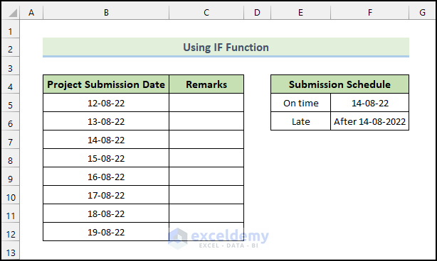
Follow these steps to see how we can use the IF functions to return a specific value if the date is between two dates in Excel.

📌 Steps:

• First of all, select the cell you want to put the value in (cell D5).
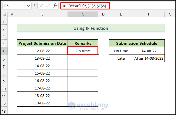
• Then write down the following formula in it.

• Next, press Enter.
• Consequently, you will get the following remark in cell D5.

• Now, select the cell again and click and drag the Fill Handle icon to the end of the column to fill the rest of the cells with this formula.
• Therefore, using the IF function, you can return a value based on the date range in Excel.

Read More: Excel If Date Is Between Range Then Return Value

2. Combining IF with AND Function

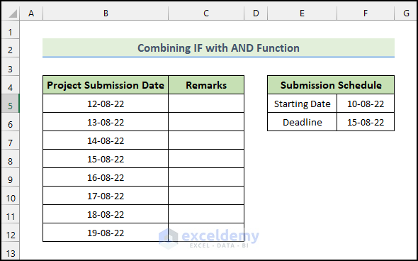
The following method is to show another method of determining the value based on the date range in Excel. Different task submission dates are included in the following dataset. Depending on the submission time, we will make different remarks. We will combine IF and AND functions in order to consider date range and outputs.

To retrieve a specific value in Excel based on date range, follow these steps.

📌 Steps:

• First of all, select the cell you want to put the value in (cell D5).
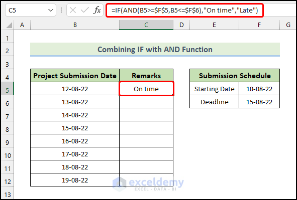
• Then write down the following formula in it.

• Next, press Enter.
• Consequently, you will get the following remark in cell D5.

• Now, select the cell again and click and drag the Fill Handle icon to the end of the column to fill the rest of the cells with this formula.
• Therefore, you can return a value based on the date range.

Read More: Return Expected Value If Date Is Greater Than Today in Excel

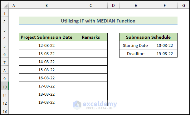
3. Utilizing IF with MEDIAN Function

It is possible to achieve the same result with the same criteria on the same dataset in another way. In this case, we’ll use the IF and MEDIAN functions to formulate the formula. The IF function takes three arguments- a condition, a value if the condition is true, and a value if it is false. Based on the condition’s outcome, it returns the value. In the meantime, the MEDIAN function returns the median of a group of numbers. Actually, that’s the middle number in a set.

To retrieve a specific value in Excel based on date range, follow these steps.

📌 Steps:

• First of all, select the cell you want to put the value in (cell D5).
• Then write down the following formula in it.

• Next, press Enter.
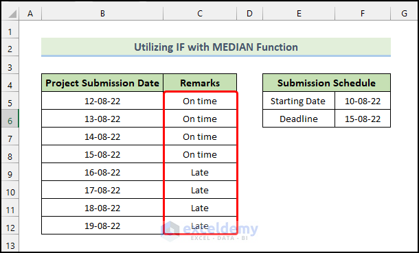
• Consequently, you will get the following remark in cell D5.

• Now, select the cell again and click and drag the Fill Handle icon to the end of the column to fill the rest of the cells with this formula.
• Therefore, you can return a value based on the date range.

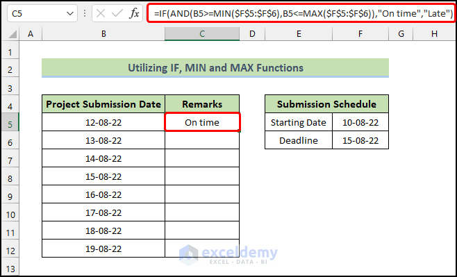
4. Applying IF, MIN and MAX Functions

Here, we will demonstrate another method to achieve the same result for the same scenarios by combining the IF, AND, MIN, and MAX functions. In the case of a condition being true, the IF function accepts a value for the true condition and a value for the false condition. Depending on the condition’s outcome, it returns a value. The AND function, on the other hand, checks that all arguments are TRUE, and returns TRUE if they all are. With the MIN function, we extract the lowest or smallest value from a set of cells or cell references. Meanwhile, the MAX function extracts the highest or largest one from the range.

To retrieve a specific value in Excel based on date range, follow these steps.

📌 Steps:

• First of all, select the cell you want to put the value in (cell D5).
• Then write down the following formula in it.

• Next, press Enter.
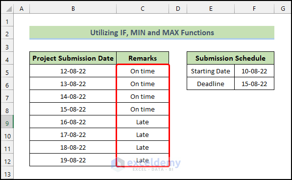
• Consequently, you will get the following remark in cell D5.

• Now, select the cell again and click and drag the Fill Handle icon to the end of the column to fill the rest of the cells with this formula.
• Therefore, you can return a value based on the date range.

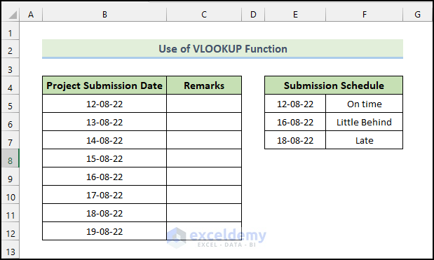
5. Use of VLOOKUP Function

Here, we will demonstrate another method by using another function in Excel called the VLOOKUP function which we can utilize to return a specific value if the dates in a specific range. The VLOOKUP function looks for a given value in the leftmost column of a given table and then returns a value in the same row from a specified column. The usage of the VLOOKUP function is more suitable to use in a scenario like the following one.

To retrieve a specific value in Excel based on date range, follow these steps.

📌 Steps:

• First of all, select the cell you want to put the value in (cell D5).
• Then write down the following formula in it.

• Next, press Enter.
• Consequently, you will get the following remark in cell D5.

• Now, select the cell again and click and drag the Fill Handle icon to the end of the column to fill the rest of the cells with this formula.
• Therefore, you can return a value based on the date range.

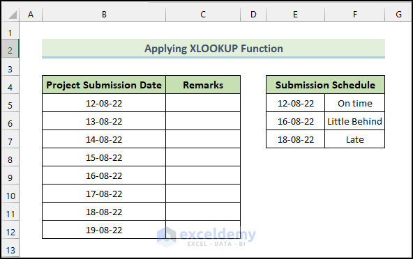
6. Applying XLOOKUP Function

If a date falls within a certain range, there is another Excel function to immediately return a result. That is how the XLOOKUP function works. The value to search for, the array or range to search in, and the array or range to return are the three arguments this function requires. Additionally, it can accept a few optional arguments.

See how we can utilize the function for the dataset by following these steps.

📌 Steps:

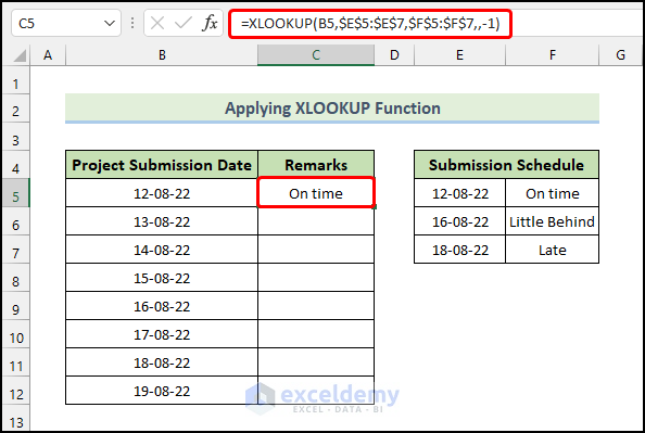
• First of all, select the cell you want to put the value in (cell D5).
• Then write down the following formula in it.

• Next, press Enter.
• Consequently, you will get the following remark in cell D5.

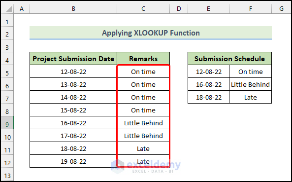
• Now, select the cell again and click and drag the Fill Handle icon to the end of the column to fill the rest of the cells with this formula.
• Therefore, you can return a value based on the date range.

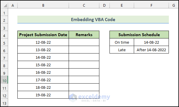
7. Embedding VBA Code

If you want to return a specific value if the date is in range in Excel, you need to use the help of VBA. The Microsoft Visual Basic for Applications (VBA) programming language is Microsoft’s event-driven programming language. To use this feature, it is necessary to have the Developer tab on your ribbon. Click here to see how you can show the Developer tab on your ribbon. Once you have that, follow these detailed steps to return a specific value if the date is in range in Excel.

📌 Steps:

⧭ Open VBA Window:

• VBA has its own separate window to work with. You have to insert the code in this window too. To open the VBA window, go to the Developer tab on your ribbon. Then select Visual Basic from the Code group.

⧭ Insert Module:

• VBA modules hold the code in the Visual Basic Editor. It has a.bcf file extension. We can create or edit one easily through the VBA editor window. To insert a module for the code, go to the Insert tab on the VBA editor. Then click on Module from the drop-down.

• As a result, a new module will be created.

⧭ Insert VBA Code:

• Now select the module if it isn’t already selected. Then write down the following code in it.

Sub Date_1()
Range("C5").Select
ActiveCell.FormulaR1C1 = "=IF(RC[-1]<=R5C6,R5C5,R6C5)"
Range("C5").Select
Selection.AutoFill Destination:=Range("C5:C12")
Range("C5:C12").Select
End Sub

• Next, save the code.

⧭ Run VBA Code:

• Afterward, close the Visual Basic window.
• Afterward, press Alt+F8.
• When the Macro dialogue box opens, select the following macro in the Macro name. Click on Run.

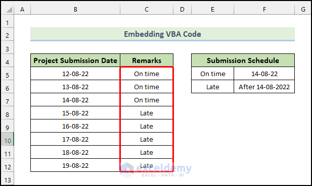
⧭ Output:

• This way, you can return a value based on the date range in Excel like in the below figure.

Sub Date_1()

Range("C5").Select
ActiveCell.FormulaR1C1 = "=IF(RC[-1]<=R5C6,R5C5,R6C5)"
Range("C5").Select

Selection.AutoFill Destination:=Range("C5:C12")
Range("C5:C12").Select

End Sub

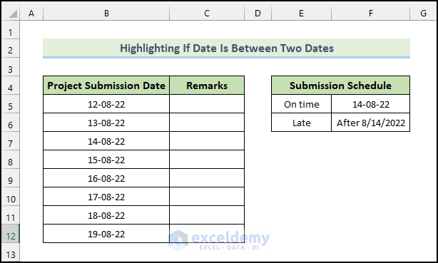
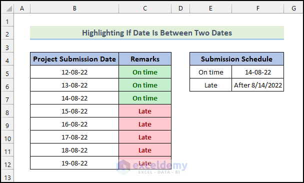
How to Highlight If Date Is Between Two Dates in Excel

Here, we demonstrate how to highlight the return specific value if the date is in between two dates in Excel. here, we will use the IF function. The following dataset contains different project submission dates.

Follow these steps to see how we can highlight the return value if the date is between two dates in Excel.

📌 Steps:

• First of all, select the cell you want to put the value in (cell D5).
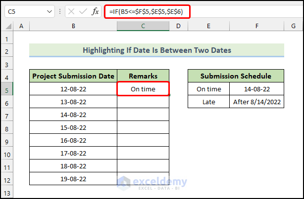
• Then write down the following formula in it.

• Next, press Enter.
• Consequently, you will get the following remark in cell D5.

• Now, select the cell again and click and drag the Fill Handle icon to the end of the column to fill the rest of the cells with this formula.
• Therefore, you can return a value based on the date range in Excel using the IF function.

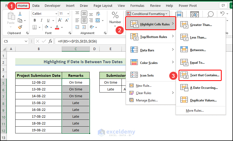
• Next, select the ranges of cells, go to the Home tab and select Conditional Formatting.
• Then, from the drop-down menu select Highlight Cells Rules.
• Afterward, from the drop-down menu select Text that Contains.

• Then, the Text That Contains dialog box will open up.
• Write On time in the first box and select your desired formatting style (here, Green File with Dark Green Text style has been selected) in the second box.
• Press OK.

• Then, follow the above process, and the Text That Contains dialog box will open up, write Late in the first box and select your desired formatting style (here, Light Red Fill with Dark Red Text style has been selected) in the second box.
• Press OK.

• Therefore, you will be able to highlight the return value based on the date range.

Download Practice Workbook

Download this practice workbook to exercise while you are reading this article. It contains all the datasets in different spreadsheets for a clear understanding. Try it yourself while you go through the step-by-step process.

Conclusion

That’s the end of today’s session. I strongly believe that from now, you may be able to return the value if the date is between two dates in Excel. If you have any queries or recommendations, please share them in the comments section below. Keep learning new methods and keep growing!

Related Articles

• How to Check If Month Is Between Two Dates in Excel
• If Cell Contains Date Then Return Value in Excel