This is an overview:
Download Practice Workbook
How to Create a Date Range in Excel
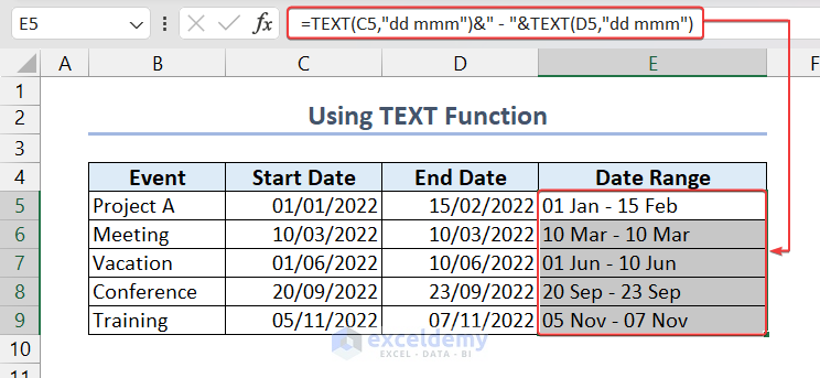
The dataset below contains the start and end dates of different events.
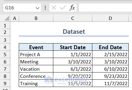
- To see the date range for each event in a single cell, use the following formula.
=TEXT(C5,"dd mmm")&" - "&TEXT(D5,"dd mmm")
Date Range in Excel – 6 Examples
Example 1 – Use the IF and the TEXT Functions to Create a Date Range if the Start or End Date Is Missing
- Use following formula to return the start date only if the end date is missing. It will return an empty string if the start date is missing.
=IF(C5<>"",TEXT(C5,"dd mmm")&IF(D5<>"","-"&TEXT(D5,"dd mmm"),""),"")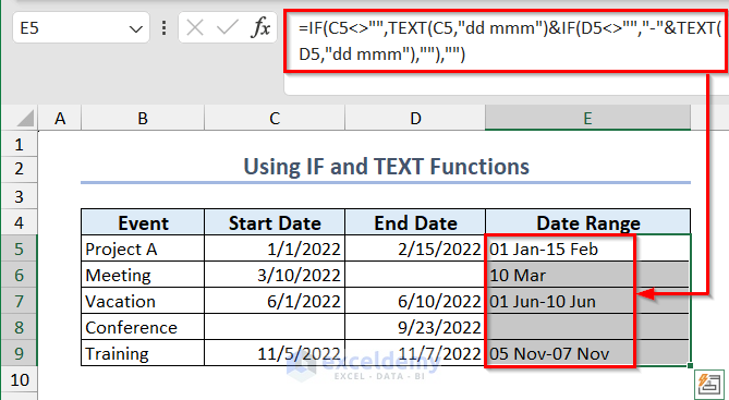
Example 2 – Create a Date Range Starting Today and Adding Number
To create a dataset in which the first Project starts today and each project takes 2 months to be completed and starts 2 days after the previous project is completed:
- Use the following formula:
=TODAY()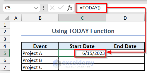
- You want the end date of Project A to be 2 months or after the start date: add 60 to C5 to get the value.
=C5+60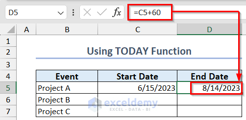
- To get the start date of Project B, add 2 to D5.
=D5+2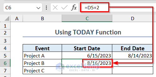
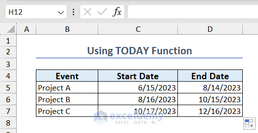
- Drag down the Fill Handle to see the result in the rest of the cells.
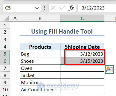
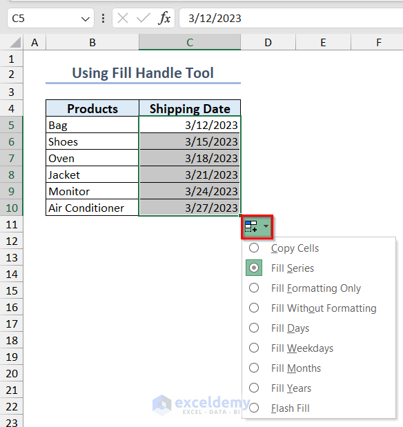
Example 3 – Create a Date Sequence in Excel
To create a date sequence with a 3-day interval:
- Enter the first 2 dates and select them.
- Drag down the Fill Handle to copy the pattern.
- Click the square box shown below to see other options to fill your dataset.
Example 4 – Count Values in a Date Range
- Use the formula:
=COUNT(C5:C10)-1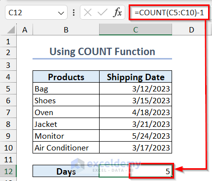
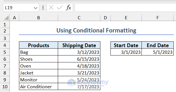
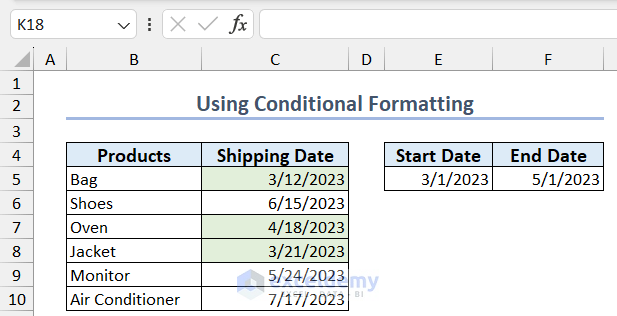
Example 5 – Highlight Values in a Date Range
The dataset contains Shipping Dates. To highlight cells between a start and end date:
- Select the values in the Shipping Date column >> go to the Home tab >> click Conditional Formatting >> select New Rule.
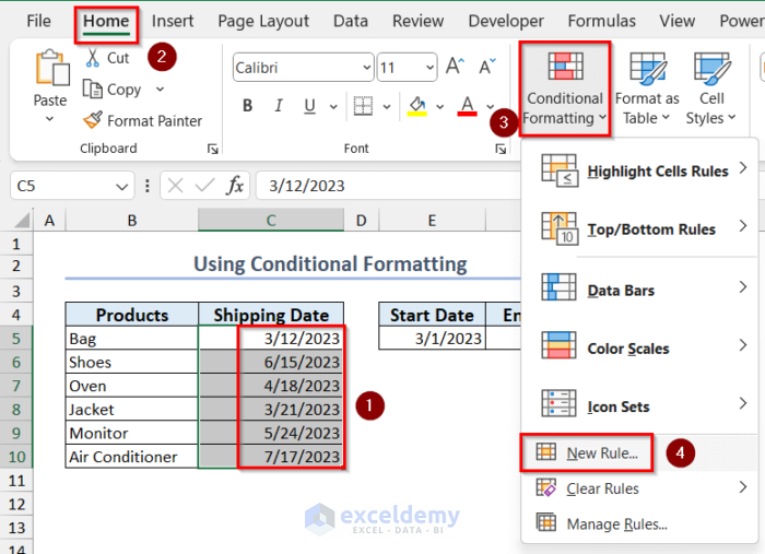
- In New Formatting Rule, select Use a formula to determine which cells to format >> enter the following formula in the box >> click Format.
=AND(C5>$E$5,C5<$F$5)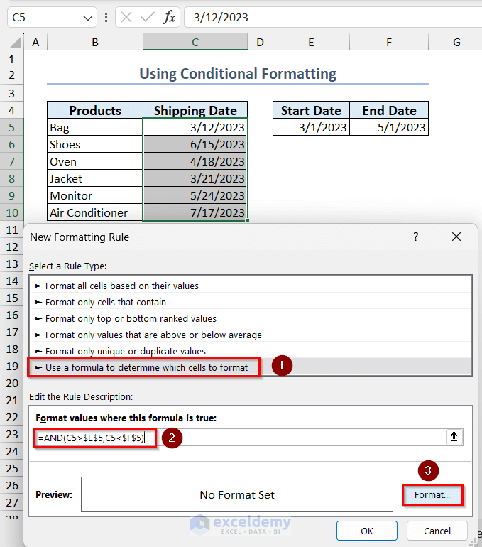
- Choose Format and click OK.
Example 6 – Get a Range from Dates in Excel
- To get the minimum value from a date range, use the MIN function:
=MIN(C5:C10)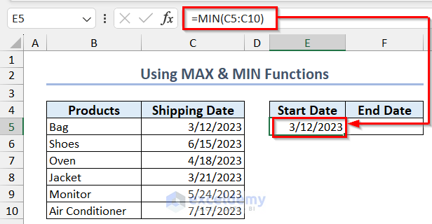
- To get the maximum value from a date range, use the MAX function:
=MAX(C5:C10)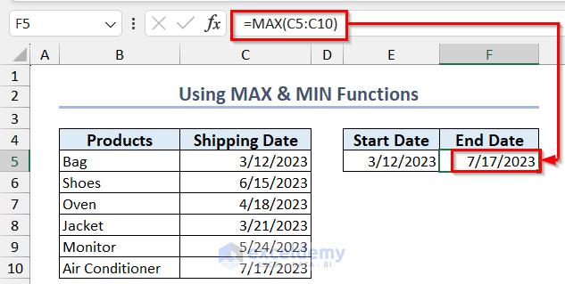
How to Use the IF Formula with a Date Range in Excel
1. Use the IF Function Only to Create a Formula
You have a list of shipment dates and want to see Shipped in Column D if the values in Column C are in the list. Otherwise, an empty string.
- Use the formula:
=IF(C5=$F$5,"Shipped",IF(C5=$F$6,"Shipped",IF(C5=$F$7,"Shippped",IF(C5=$F$8,"Shipped",IF(C5=$F$9,"Shipped",IF(C5=$F$10,"Shipped",""))))))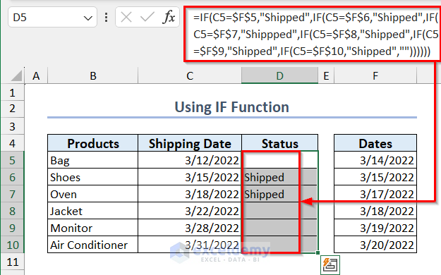
2. Use the AND and the IF Functions
- Use the following formula to return Shipped if the date is between a range. Otherwise, it will return Pending.
=IF(AND(C5>=$F$8,C5<=$G$8),"Shipped","Pending")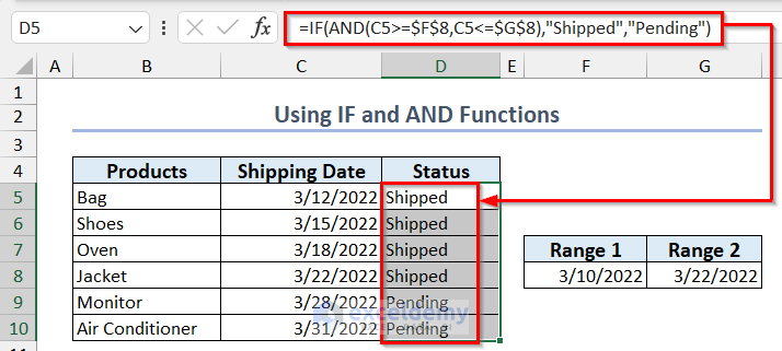
3. Use the OR and the IF Functions
To check if a date belongs to a date range:
- Use the formula:
=IF(OR(C5=$F$5,C5=$F$6,C5=$F$7,C5=$F$8,C5=$F$9,C5=$F$10),"Will be Delayed","")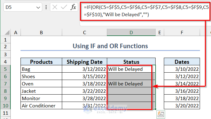
4. Use the IF and the COUNTIF Functions
- Use the formula:
=IF(COUNTIF($F$5:$F$10,C5),"Shipped","")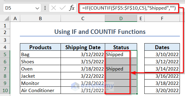
5. Use the IF and the TODAY Functions
- Use the formula to determine the order status based on the value in Column C compared to the current date.
=IF(C5<=TODAY(),"Shipped","Pending")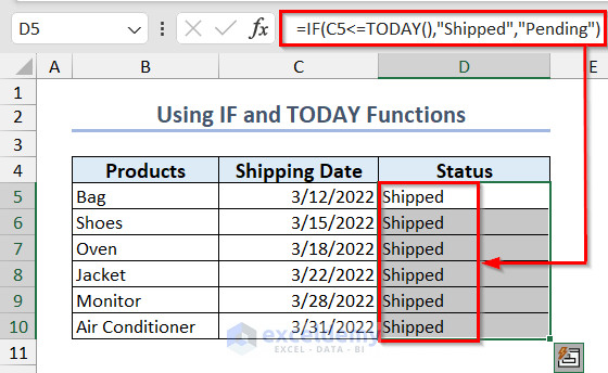
6. Using the IF and the SORT Functions
To check if a date range is in a specified order:
- Use the following formula. It will return Yes if the date range is sorted and No if it is not.
=IF(SUM(--(C5:C10<>SORT(C5:C10,1,1,0)))=0,"YES","NO")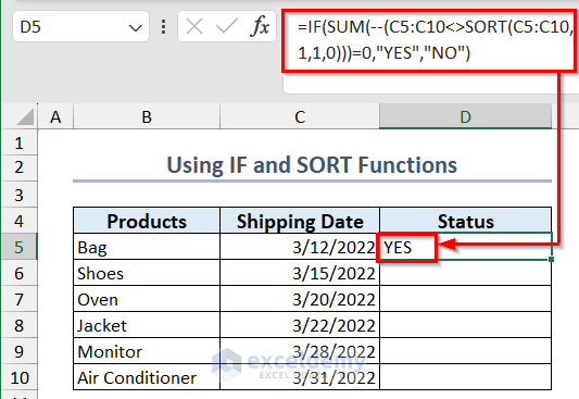
Read More: How to Use IF Formula for Date Range in Excel
How to Use the SUMIFS Function with a Date Range in Excel
1. Use the SUMIFS Function Between Two Dates
The dataset contains product prices and shipping dates. To sum the prices with a shipping date between two dates:
- Use the formula:
=SUMIFS(C5:C10, D5:D10, ">="&F5, D5:D10, "<="&G5)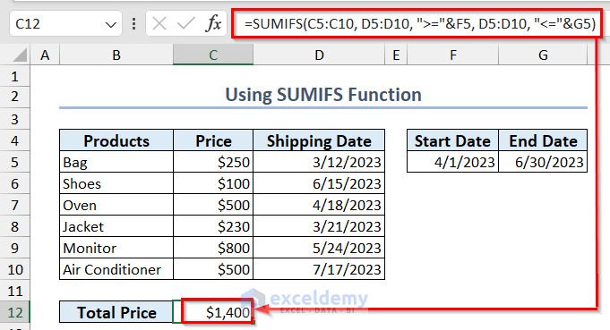
2. Sum Within a Dynamic Range using the current Date
To sum values based on a date range between today and 10 days after the current date:
- Use the formula:
=SUMIFS(C5:C10, D5:D10, "<"&TODAY(), D5:D10, ">="&TODAY()-G5)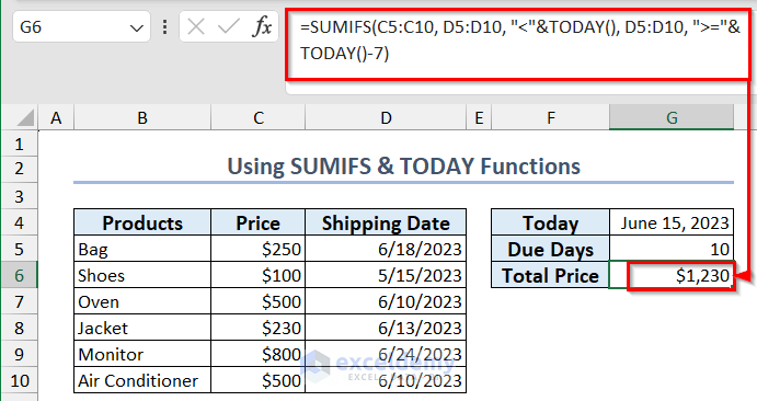
3. Sum Between Two Dates using Another Criterion
To calculate the sum of product prices with a shipping date between two given dates and containing the word Black in the product name:
- Use the formula:
=SUMIFS(C5:C10, D5:D10, ">="&F5, D5:D10, "<="&G5,B5:B10,"Black*")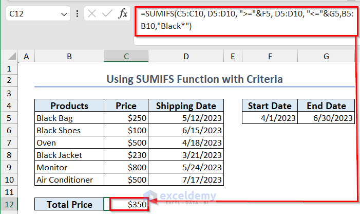
The Excel SUMIFS Function Between Dates is Not Working
Solutions:
- Check the date and number format.
- Make sure ranges are the same size.
Excel Date Range: Knowledge Hub
- How to Pull Data from a Date Range in Excel
- How to Calculate Average If within Date Range in Excel
- How to Find Max Date in Range with Criteria in Excel
- VLOOKUP Date Range and Return Value in Excel
- How to Use Formula for Past Due Date in Excel
- How to Calculate Due Date with Formula in Excel
<< Go Back to Date-Time in Excel | Learn Excel
Get FREE Advanced Excel Exercises with Solutions!
