VLOOKUP Date Range and Return Value in Excel: 4 Methods

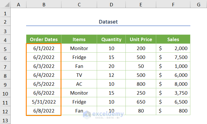
Let’s introduce today’s dataset where the name of the Items is provided along with Order Dates, Unit Price, Quantity and Sales.

Method 1 – VLOOKUP a Date within Date Range and Return Value

From the sample dataset, let’s say the lookup date within the date range (i.e. Order Dates) is in the D14 cell. Then, you want to return the value of the Sales of the corresponding cell (Lookup Order Date).

Use the following formula in the D15 cell:

Here, D14 is the lookup order date, B5:F12 is the table array, 5 is the column index number (i.e. going to the fifth column to the right of the match result), and finally TRUE is for approximate matching.

Read More: How to Use Formula for Past Due Date in Excel

Method 2 – Find a Single Output Dealing with Two Dates

Let’s saw we have to find sales between two dates.

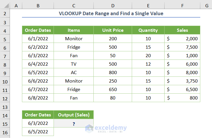
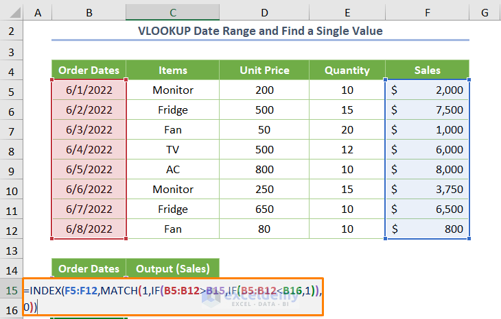
• Insert the following formula in the C15 cell:

Here, F5:F12 is the cell range for the Sales data, B5:B12 is the cell range for Order Dates, B15 is a date within the date range and B16 is another date within the date range.

In the above formula, the IF logical function returns 1 if the cell fulfills the criteria (greater than but less than). Next, the MATCH function provides the location of the matched values. Finally, the INDEX returns the value of the Sales that fulfills all criteria.

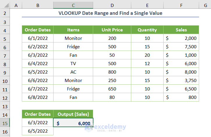
• When you press Enter, you’ll get the following output.

Note: If you want to use this method for a specific date within the date range, you can find that also. In that case, you have to insert the same date instead of the second date.

Method 3 – VLOOKUP Date Range with Multiple Criteria and Return Multiple Values

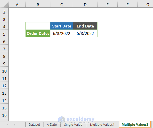
Step 01: Specifying the Start and End Dates

Initially, you have to specify the Start Date and End Date. In such a situation, using the Name Manager might be useful for updating the data frequently.

• Type two dates in two different cells as shown in the following picture.

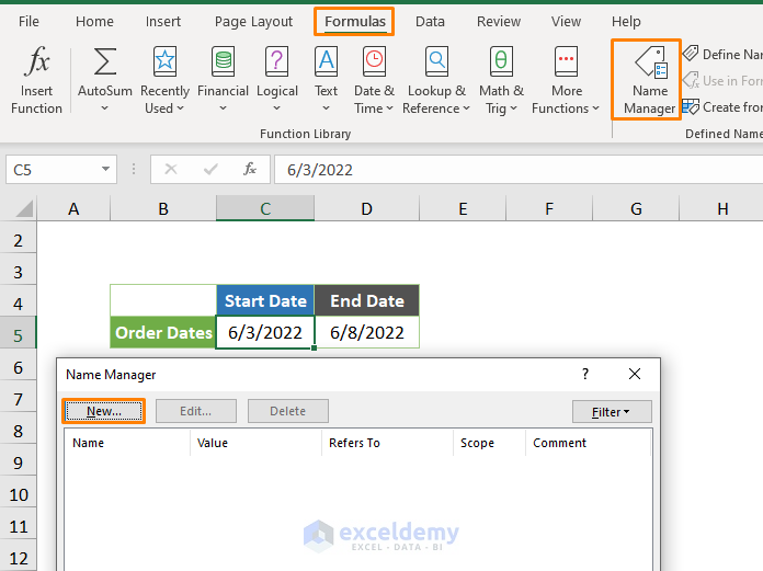
• Select the C5 cell which shows the Start Date, and choose the Name Manager from the Formulas tab.
• Click on the New option.

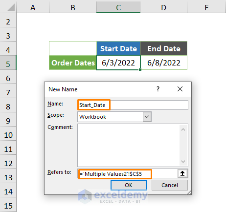
• Input the name as Start_Date.
• Repeat the same process for D5 (in the example) and name it End Date.

Step 02: Dealing with the Multiple Criteria of the Date Range

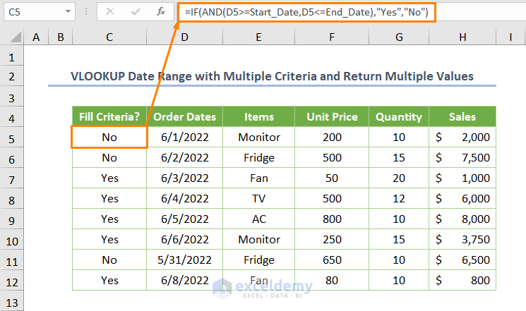
• Put the following formula into the first result cell:

Here, AND function returns dates that fulfill two criteria. Furthermore, if the criteria are fulfilled, the IF function returns Yes. Else, it will return No. The cell D5 contains the order date you’re comparing.

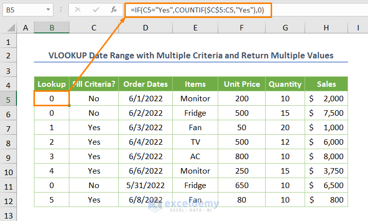
Step 03: Counting the Lookup Value

• The following combined formula utilizes the IF and COUNTIF functions to count the lookup value if the cell fulfills criteria (matches Yes). Else, it will return 0:

Here, C5 is the starting cell of the Lookup field.

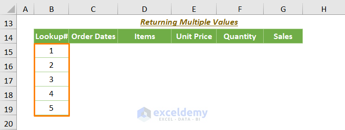
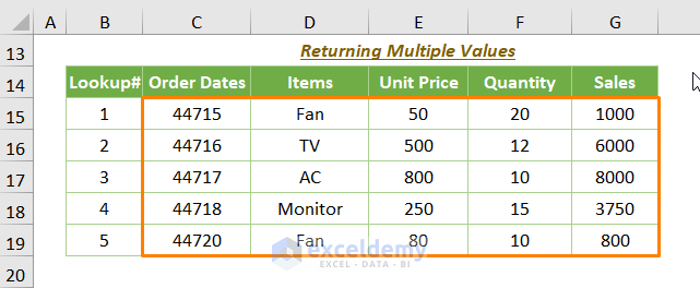
Step 04: Returning Multiple Values

• Copy the name of all fields (not the values) in the previous step except the Fill Criteria.
• Enter the lookup value sequentially in the Lookup# field.

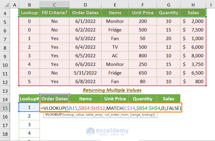
• Go to the C15 cell and insert the following formula.

$B15 is the value of the Lookup# field, $B$4:$H$12 is the table array, C$14 is the lookup value, $B$4:$H$4 is the lookup array, 0 is for the exact matching. The MATCH function finds the column index number actually for the VLOOKUP function. Finally, the VLOOKUP function returns a matched value of the Order Dates.

You have to specify a fixed reference with the dollar sign ($) carefully, or you won’t get the desired output.

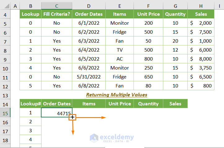
• Press Enter, and you’ll get the output is 44715. This is how Excel stores dates in a numerical format.
• Drag the plus sign to the adjacent columns until the Sales and the below cells until the lookup value is 5 (use the Fill Handle Tool).

• You should get the following output.

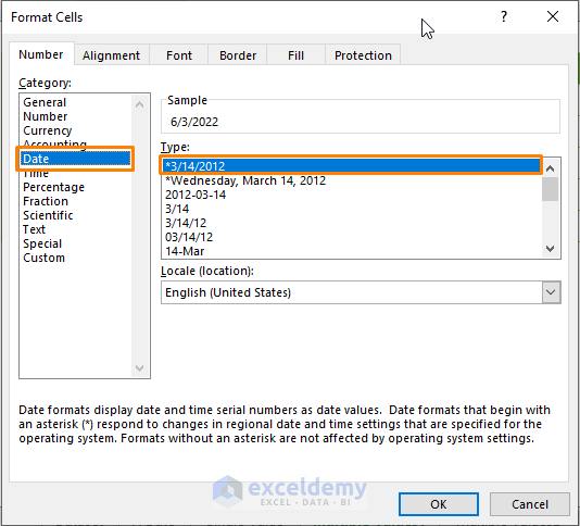
• Select the cell range C15:C19 and press Ctrl + 1 to open the Format Cells option.

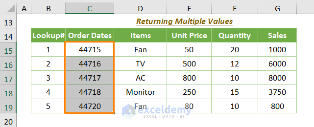
• Choose the Date format.

Read More: How to Use IF Formula for Date Range in Excel

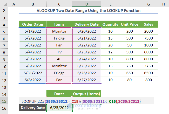
Method 4 – VLOOKUP Two Date Ranges Using the LOOKUP Function

For this example, we have added an individual column namely Delivery Date and need to find the specific item that meets both given dates.

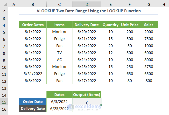
Insert the following formula into the result cell:

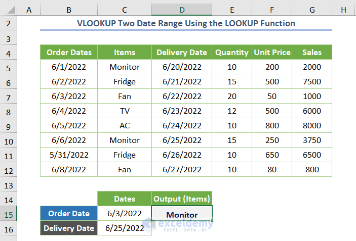
Here, $B$5:$B$12 is the cell range of the Order Dates, $D$5:$D$12 is the cell range for the Delivery Dates, C15 is an order date and C16 is delivery date. Finally, $C$5:$C$12 is the cell range for the Items.

After inserting the formula, you’ll get the following output.

Download Practice Workbook

Related Articles

• How to Calculate Average If within Date Range in Excel
• How to Pull Data from a Date Range in Excel
• How to Find Max Date in Range with Criteria in Excel

<< Go Back to Date Range | Date-Time in Excel | Learn Excel