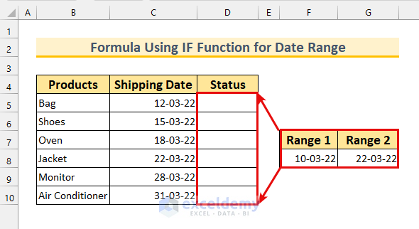
We’ve taken a sample dataset with three columns: Products, Shipping Date, and Status. We’ll check if a date falls between a range, equals a range, and a few other criteria.
Method 1 – Creating a Formula with the IF Function Only for a Date Range in Excel
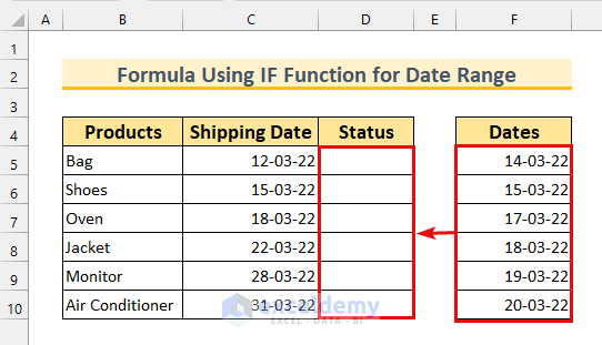
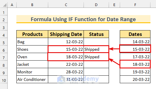
We’ll check if the Shipping Date is equal to any values in the Dates range.
Steps:
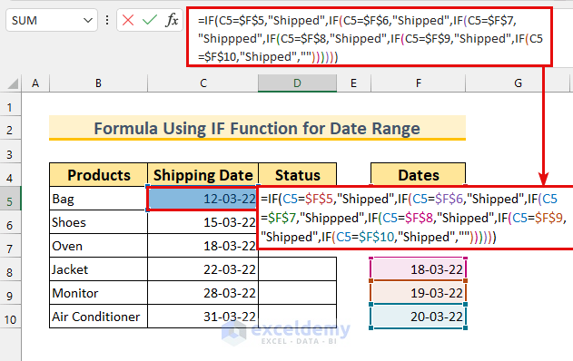
- Use the following formula in cell D5.
=IF(C5=$F$5,"Shipped",IF(C5=$F$6,"Shipped",IF(C5=$F$7,"Shippped",IF(C5=$F$8,"Shipped",IF(C5=$F$9,"Shipped",IF(C5=$F$10,"Shipped",""))))))This formula checks if the value of cell C5 equals any of the values from the Dates range. If a match is found, it will output “Shipped;” otherwise, it will leave the cell blank.
- Press Enter.
- Use the Fill Handle to copy the formula to the other cells.
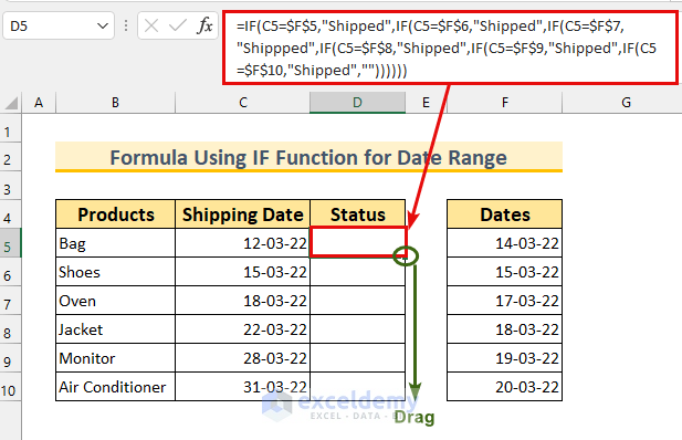
- The cells C6 and C7 matched with the Dates range. Their status is Shipped.
Read More: How to Pull Data from a Date Range in Excel
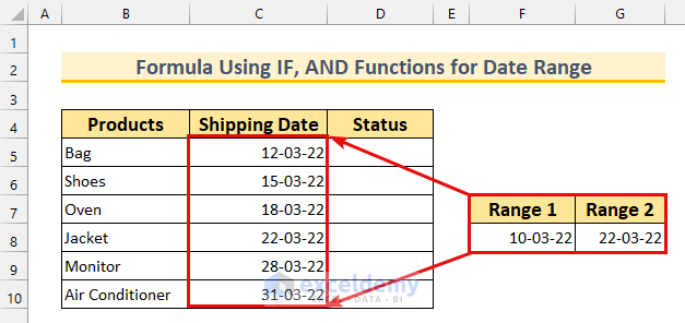
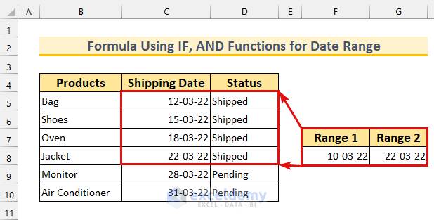
Method 2 – Applying AND and IF for a Date Range in Excel
The dates between 10 March and 22 March will set the product Status to Shipped.
Steps:
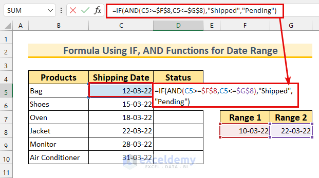
- Use this formula in cell D5.
=IF(AND(C5>=$F$8,C5<=$G$8),"Shipped","Pending")This formula is checking the date from cell C5 against cells F8 and G8. If the value is in between the range then it will show “Shipped.” Otherwise, “Pending” will be shown. The AND function ensures that IF will return the TRUE value only if both conditions are met.
- Press Enter.
- Drag down the Fill Handle to AutoFill the formula.
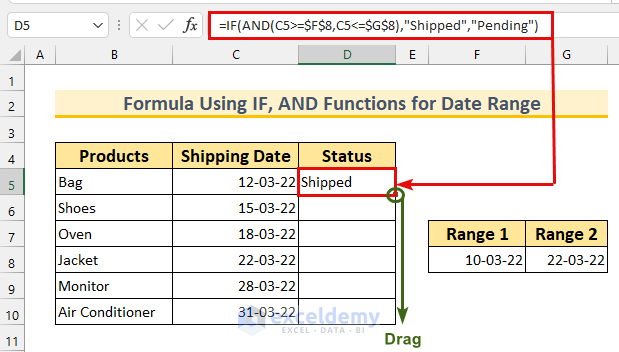
- Here’s the result.
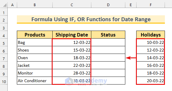
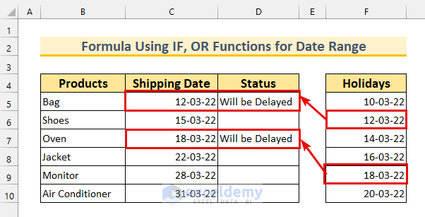
Method 3 – Combining Excel OR and IF Functions for Date Range
If the Shipping Date falls on one of the Holidays, the Status will show Will be Delayed.
Steps:
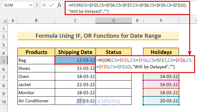
- Use the following formula in cell D5.
=IF(OR(C5=$F$5,C5=$F$6,C5=$F$7,C5=$F$8,C5=$F$9,C5=$F$10),"Will be Delayed","")The OR function returns TRUE if one (or more) of the conditions are satisfied, where each condition is an individual check for cell C5 against each of the cells in the F column. Then, IF uses that output to display the result.
- Press Enter.
- AutoFill the formula to the rest of the cells.
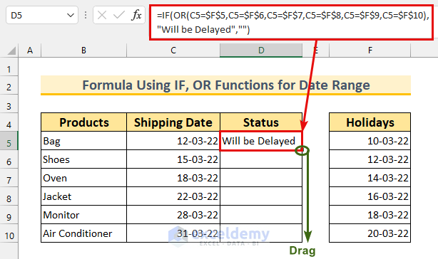
- Here are the results.
Read More: How to Calculate Average If within Date Range in Excel
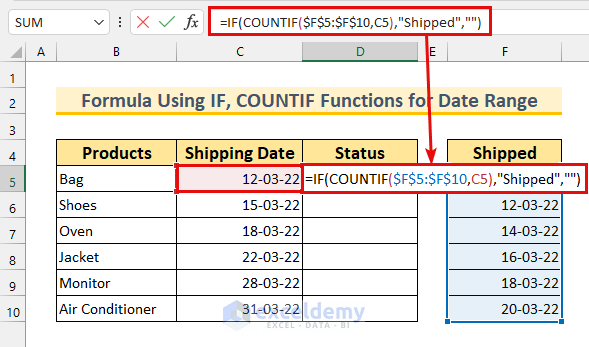
Method 4 – Combining Excel Functions to Create a Formula for a Date Range
We’re going to check if the products are shipped based on if the dates match with a value in the Shipped column.

Steps:
- Use the formula from below in cell D5.
=IF(COUNTIF($F$5:$F$10,C5),"Shipped","")The COUNTIF function counts the number of instances of the value from C5 appearing in the range $F$5:$F$10. The IF function considers a value of 1 or greater as TRUE and will show “Shipped” for it. Otherwise, it leaves the cell blank.
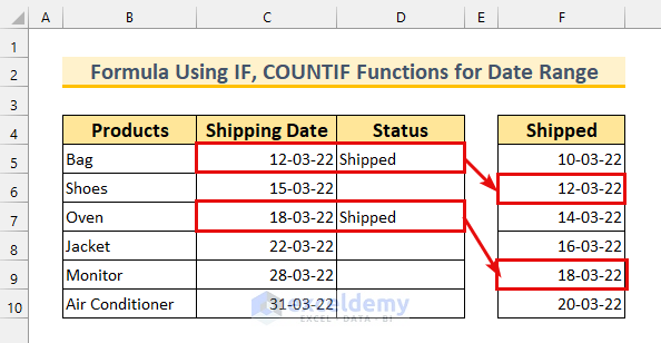
- Hit Enter and AutoFill the formula to the cell C6:C10 range.
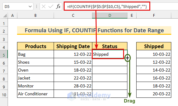
Here’s the result.
Read More: How to Find Max Date in Range with Criteria in Excel
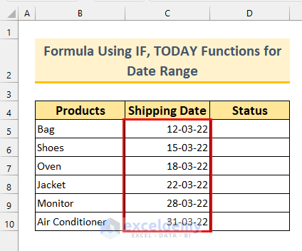
Method 5 – Creating a Formula for a Date Range with IF and TODAY Functions
If the Shipping Date values are less or equal to today’s date, we will output “Shipped.” Otherwise, the status becomes Pending.
Steps:
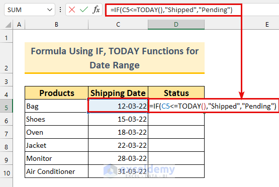
- Enter the following formula into cell D5.
=IF(C5<=TODAY(),"Shipped","Pending")We’re checking if the value from cell C5 is less or equal to today’s date. If it is, then “Shipped” will be the output in cell D5.
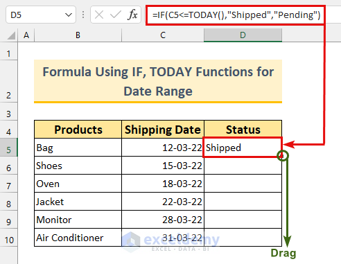
- Press Enter. The today’s date is March 12 (as of time of writing) which is less than March 23, 2022. We’ve got the value “Shipped”.
- AutoFill the formula to cell range C6:C10.
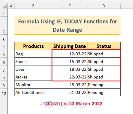
- Here are the results.
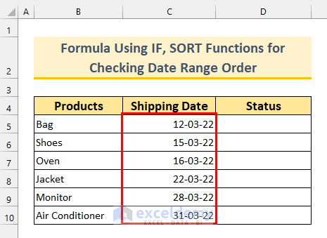
Method 6 – Joining Excel IF-SORT Functions to Check the Date Range Order
We’ll check whether the dates are in ascending order.
Steps:
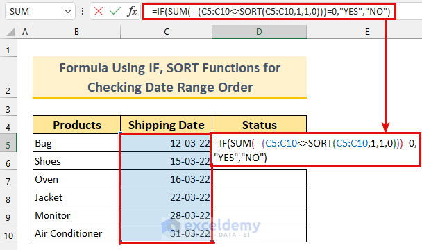
- Insert the following formula in cell D5.
=IF(SUM(--(C5:C10<>SORT(C5:C10,1,1,0)))=0,"YES","NO")Formula Breakdown
- SORT(C5:C10,1,1,0) is sorting the row range C5:C10 in ascending order.
- C5:C10<>SORT(C5:C10,1,1,0) is comparing the cell values with the sorted values.
- SUM(–(C5:C10<>SORT(C5:C10,1,1,0)) —> becomes
- Output: {0}.
The formula will reduce to-
- IF(TRUE,”YES”,”NO”).
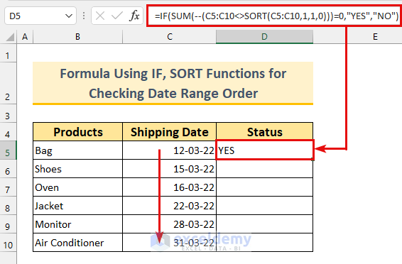
- Output: YES.
- Press Enter. The dates are in ascending order, so we got “YES” as the output.
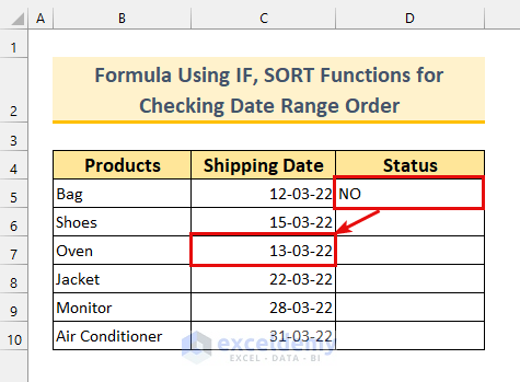
- We’ve changed a date. Thus, we received “NO” as the output.
Download the Practice Workbook
Related Articles
<< Go Back to Date Range | Date-Time in Excel | Learn Excel
Get FREE Advanced Excel Exercises with Solutions!
