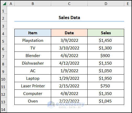
We’ll use a simple sales dataset to demonstrate how you can pull data from a date range.
Method 1 – Using the FILTER Function
Steps:
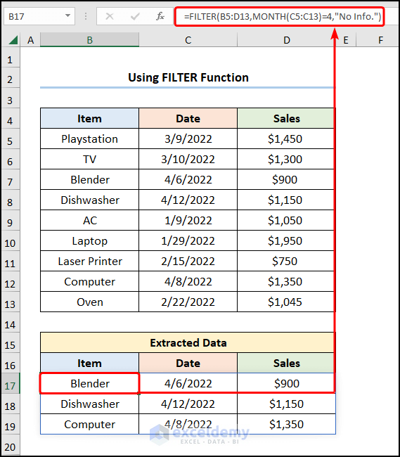
- Go to cell B17 and enter the formula below.
=FILTER(B5:D13,MONTH(C5:C13)=4,"No Info.")
- FILTER(B5:D13,MONTH(C5:C13)=4,”No Info.”) → filter a range or array. Here, B5:D13 is the array argument, while MONTH(C5:C13)=4 is the include argument that selects the values corresponding to the month of “April”. “No Info.” is the optional if_empty argument that is returned by the function if there are no matches.
Note: The FILTER function is available on Microsoft Excel 365, if you’re using an older version of Excel, then please check the second method.
Read More: How to Use IF Formula for Date Range in Excel
Method 2 – Combining INDEX, MATCH, SMALL, IF, ROW, and COLUMN Functions
Steps:
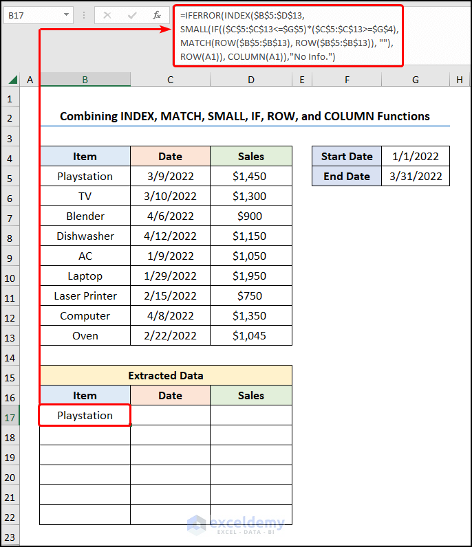
- Move to the B17 cell and insert the following formula.
=IFERROR(INDEX($B$5:$D$13, SMALL(IF(($C$5:$C$13<=$G$5)*($C$5:$C$13>=$G$4), MATCH(ROW($B$5:$B$13), ROW($B$5:$B$13)), ""), ROW(A1)), COLUMN(A1)), "No Info.")
- COLUMN(A1) → returns the column number of a cell reference.
- Output → 1
- ROW(A1) → returns the serial number of a reference.
- Output → 1
- MATCH(ROW($B$5:$B$13), ROW($B$5:$B$13)) → returns the relative position of an item in an array matching the given value. Here, ROW($B$5:$B$13) is the lookup_value argument that refers to the “Item” column. Following, ROW($B$5:$B$13) represents the lookup_array argument from where the value is matched.
- Output → {1;2;3;4;5;6;7;8;9}
- IF(($C$5:$C$13<=$G$5)*($C$5:$C$13>=$G$4), MATCH(ROW($B$5:$B$13), ROW($B$5:$B$13)), “”) → checks whether a condition is met and returns one value if TRUE and another value if. Here, ($C$5:$C$13<=$G$5)*($C$5:$C$13>=$G$4) is the logical_test argument which prompts the IF function to return the value from MATCH(ROW($B$5:$B$13), ROW($B$5:$B$13)) (value_if_true argument) otherwise it returns blank “” (value_if_false argument).
- Output → {1;2;””;””;5;6;7;””;9}
- SMALL(IF(($C$5:$C$13<=$G$5)*($C$5:$C$13>=$G$4),MATCH(ROW($B$5:$B$13), ROW($B$5:$B$13)), “”), ROW(A1)) → becomes
- SMALL({1;2;””;””;5;6;7;””;9}, 1) → returns the kth smallest value in data set.
- Output → {1}
- INDEX($B$5:$D$13, SMALL(IF(($C$5:$C$13<=$G$5)*($C$5:$C$13>=$G$4), MATCH(ROW($B$5:$B$13), ROW($B$5:$B$13)), “”), ROW(A1)), COLUMN(A1)) → becomes
- INDEX($B$5:$D$13, 1, 1) → returns a value at the intersection of a row and column in a given range. In this expression, the $B$5:$D$13 is the array argument which is the “Item” column. Next, 1 is the row_num argument that indicates the row location, while 1 is the column_num argument that indicates the column location.
- Output →”Playstation”
- IFERROR(INDEX($B$5:$D$13, SMALL(IF(($C$5:$C$13<=$G$5)*($C$5:$C$13>=$G$4), MATCH(ROW($B$5:$B$13), ROW($B$5:$B$13)), “”), ROW(A1)), COLUMN(A1)), “No Info.”) → becomes
- IFERROR(“Playstation”, “No Info.”) → returns value_if_error if the expression has an error and the value of the expression itself otherwise. Here, “Playstation” is the value argument, and “No Info.” is the value_if_error argument.
- Output → “Playstation”
- Here’s a GIF overview.
Read More: VLOOKUP Date Range and Return Value in Excel
Method 3 – Using the Date Filter Feature
Steps:
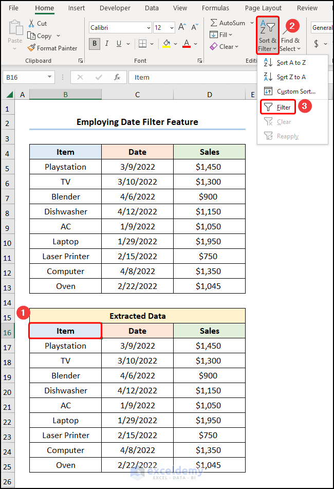
- Navigate to cell B16, click the Sort & Filter drop-down, and choose Filter.
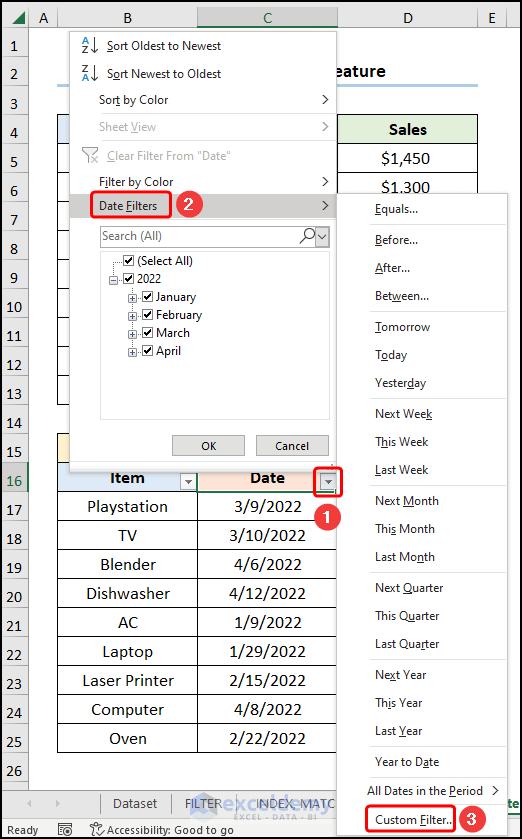
- Click the Down-arrow button, jump to Date Filters, and select Custom Filter.
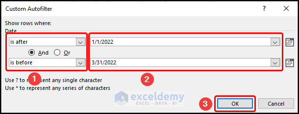
- Select the “Date is after 1/1/2022 and is before 3/31/2022” criteria and hit OK.
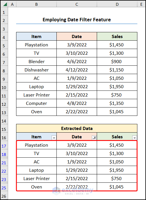
The results will look like the image below for the sample.
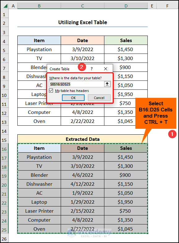
Method 4 – Utilizing an Excel Table
Steps:
- Choose the B16:D25 array.
- Press the CTRL + T shortcut keys to insert a Table.
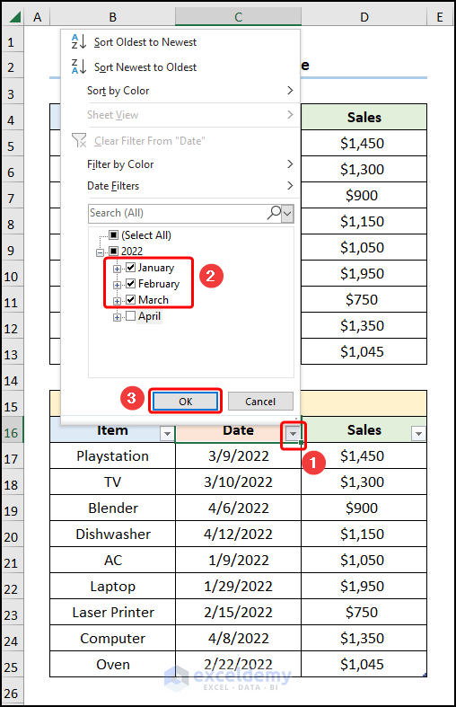
- Press the Down-arrow button.
- Choose the months “January”, “February”, and “March”.
- Click OK.
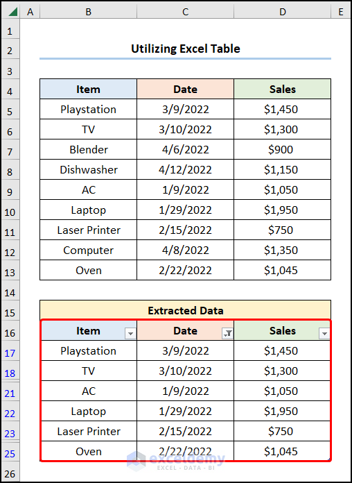
The final table should look like the picture below.
Similar Readings
- How to Calculate Average If within Date Range in Excel
- How to Find Max Date in Range with Criteria in Excel
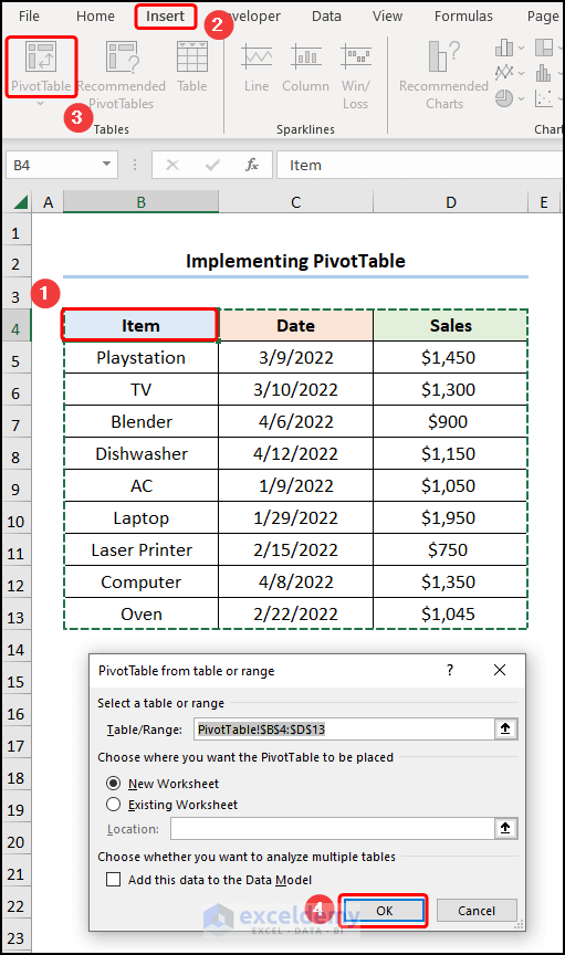
Method 5 – Implementing a PivotTable
Steps:
- Go to the B4 cell.
- Click on Insert, press the PivotTable button, select the New Worksheet option, and hit OK.
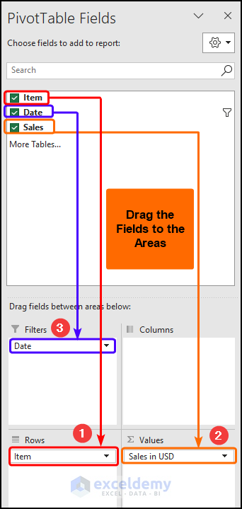
- Drag the “Item”, “Date”, and “Sales” Fields into the “Rows”, “Values”, and “Filter” Areas, respectively.
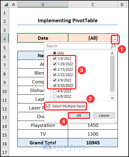
- Press the Down-arrow button on (All), tick the Select Multiple Items box, choose the dates you need, and click OK.
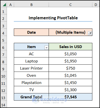
The end results should look like the figure below.
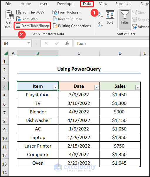
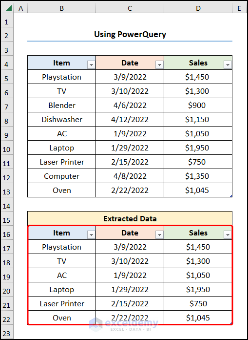
Method 6 – Using PowerQuery
Steps:
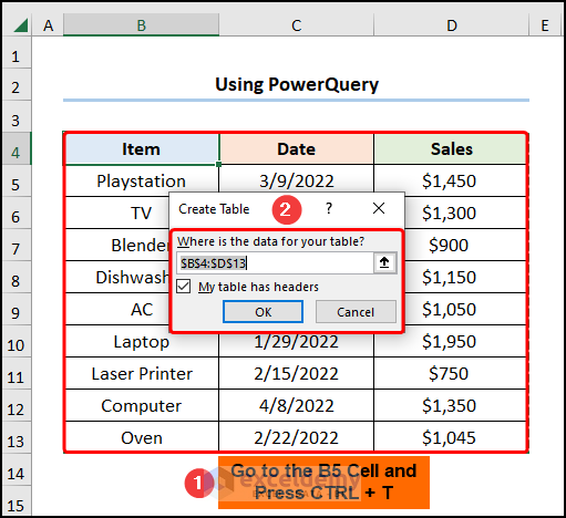
- Go to the B5 cell and press CTRL + T to convert the dataset into a Table.
- Move to the Data tab and choose From Table/Range.
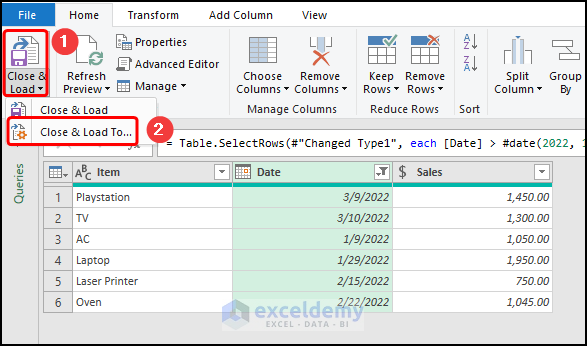
- Follow the steps in the GIF for a live demonstration to filter the dated range.
- Press the Close & Load drop-down and choose the Close & Load To option.
- Check the Existing worksheet button, enter the B16 cell reference in the location box, and press OK.
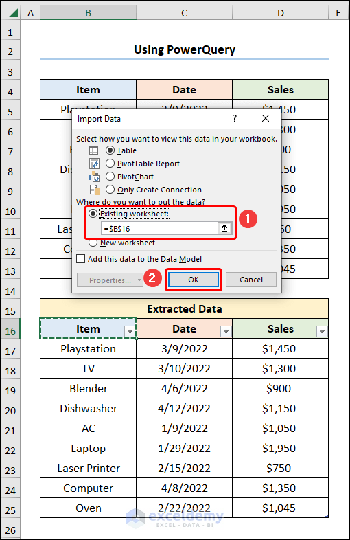
Here’s the output in the sample.
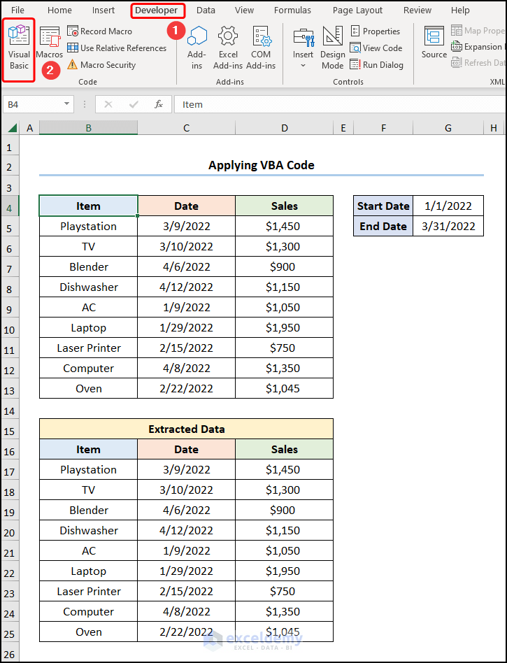
Method 7 – Applying VBA Code
Steps:
- Navigate to the Developer tab and click the Visual Basic button.
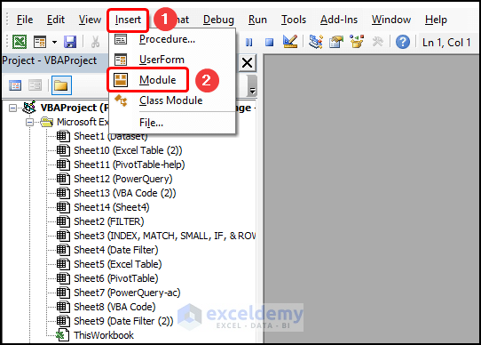
- Go to the Insert tab and select Module.
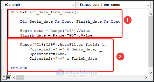
Copy the code below and paste it into the window as shown below.
Sub Extract_date_from_range()
    Dim Begin_date As Long, Finish_date As Long
    Begin_date = Range("G4").Value
    Finish_date = Range("G5").Value
    Range("C16:C25").AutoFilter field:=1, _
        Criteria1:=">=" & Begin_date, _
        Operator:=xlAnd, _
        Criteria2:="<=" & Finish_date
End Sub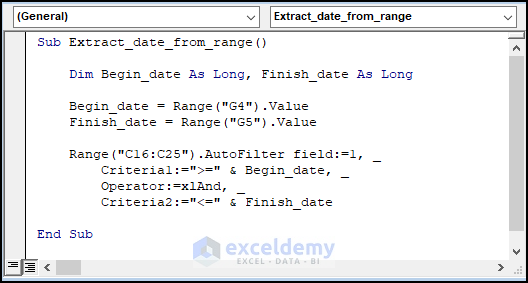
The VBA code used to extract data from a date range.
- The sub-routine is given a name, here it is Extract_date_from_range().
- Define the variables Begin_date and Finish_date; assign the Long data type.
- Use the Range.Value to set the cell references for the starting and ending dates, in this case, “1/1/2022” and “3/31/2022”.
- Apply the Range.AutoFilter to filter the dates in between the starting and ending dates.
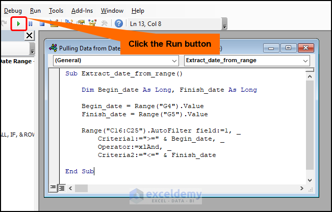
- Click the Run button to execute the macro.
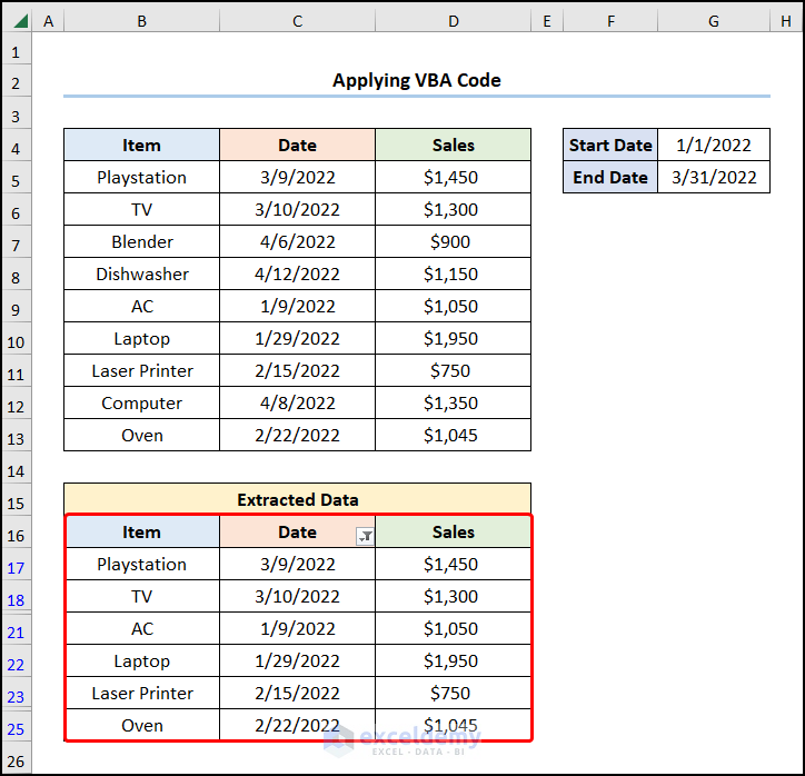
The results should look like the screenshot below.
Read More: How to Use Formula for Past Due Date in Excel
Download the Practice Workbook
<< Go Back to Date Range | Date-Time in Excel | Learn Excel
Get FREE Advanced Excel Exercises with Solutions!
