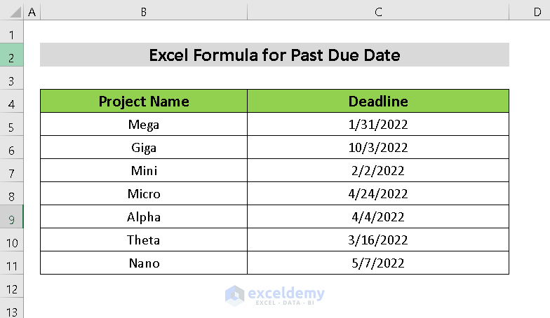
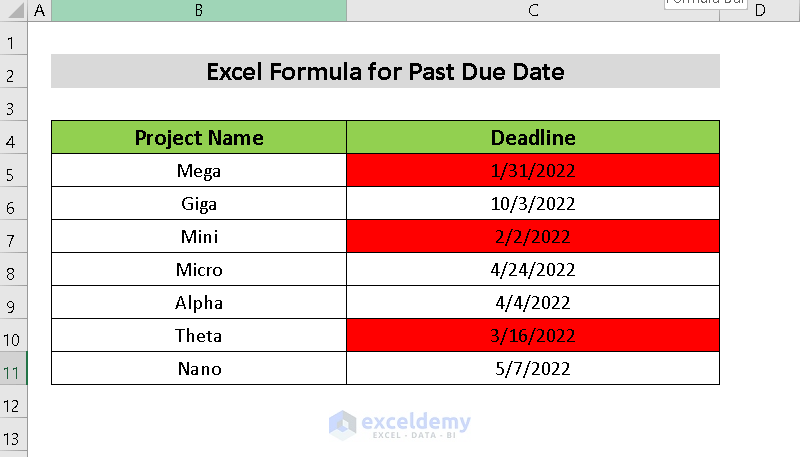
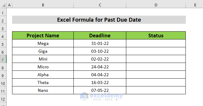
How to Use Formula for Past Due Date in Excel (3 Methods)

To demonstrate how to use formulas for due dates, we’ll use a dataset containing data titled Project Name and Deadline.

How to Use a Formula for Past Due Date in Excel: 3 Ways

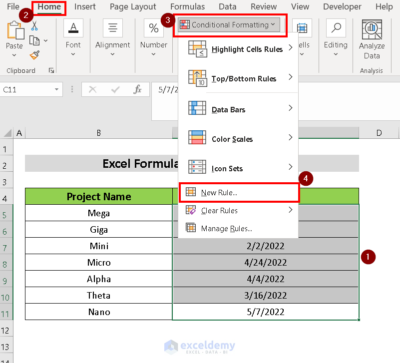
Method 1 – Using the Excel TODAY Function in Conditional Formatting for Past Due Date

Steps:

Select all the cells containing dates. We have selected cells C5:C11.
Choose Home from the ribbon.
Select Conditional Formatting and New Rule.

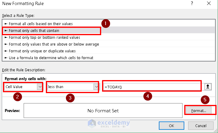
A dialog box will appear. Choose Format only cells that contain from Select a Rule Type.
For the Format only cells with, select Cell Value and less than
Insert =TODAY() in the textbox.
Select Format.

Another dialog box will appear named Format Cells. Select the Fill tab and choose a color.
Press OK.

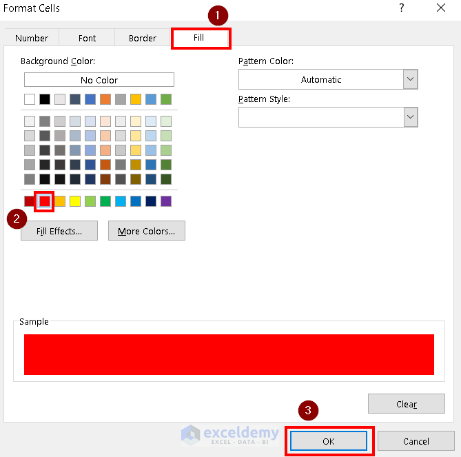
Press OK again.

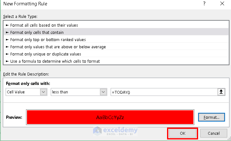
The formula will be applied and past due dates will be identified.

Method 2 – Applying Excel IF and ISBLANK Functions for Past Due Date

Steps:

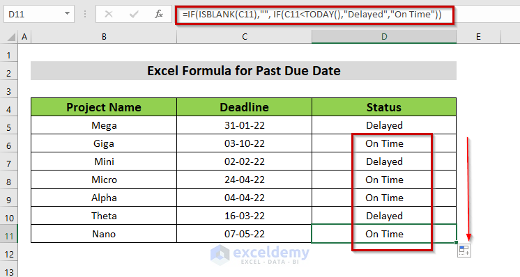
Select the cell D5 and input the following formula:

=IF(ISBLANK(C5),"", IF(C5<TODAY(),"Delayed","On Time"))

The ISBLANK Function is used to check if the selected cell is blank or not. A condition is applied using IF Function which gives the Delayed output for value lower than today compared with the selected cell value and On Time output for the rest.

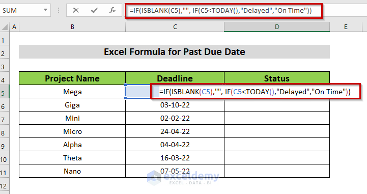
Press Enter.

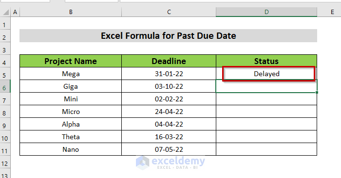
Use the Fill Handle to AutoFill the rest of the column.

Similar Readings

Method 3 – Using Excel Combined Functions for Past Due Date

Steps:

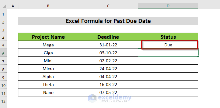
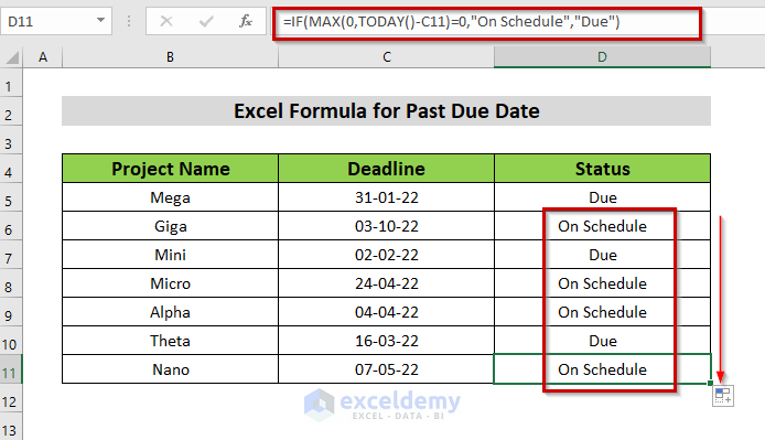
Insert the following formula in D5 to check cell C5’s due date:

=IF(MAX(0,TODAY()-C5)=0,"On Schedule","Due")

The MAX Function returns the largest value and ignores the empty cells. A condition is applied here using IF Function, where the function will output On Schedule or Due if today’s date is higher than the comparison cell.

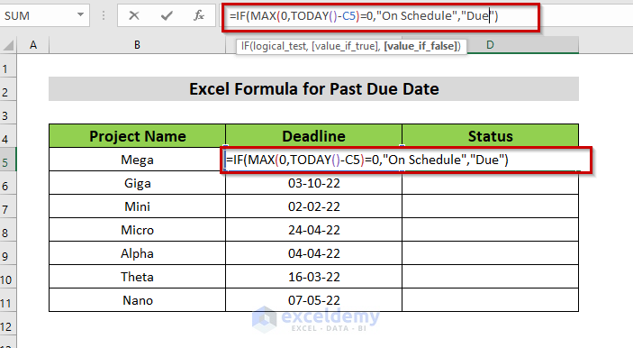
Press Enter.

For AutoFill, use the Fill Handle.

Practice Section

Use the practice workbook to practice, inputting your own values.

Download the Practice Workbook

Excel Formulas for Past Due Date.xlsx

<< Go Back to Date Range | Date-Time in Excel | Learn Excel

Get FREE Advanced Excel Exercises with Solutions!

Private Sub Worksheet_Change(ByVal Target As Range) If Target.Address = "$A$1" Then ' Change the cell reference to the desired cell triggering the alert MsgBox "Alert: Cell A1 has been changed!" ' Customize the alert message as needed End If End Sub

Sub BlinkText() Dim rng As Range Set rng = Range("A1") ' Change the cell reference to the desired cell to blink For i = 1 To 5 ' Number of times to blink rng.Font.Color = RGB(255, 0, 0) ' Change font color to red Application.Wait Now + TimeValue("00:00:01") ' Wait for 1 second rng.Font.Color = RGB(0, 0, 0) ' Change font color back to black Application.Wait Now + TimeValue("00:00:01") ' Wait for 1 second Next i End Sub

6 Comments

ATEEB Feb 3, 2023 at 4:20 PM

Dear Sir,
Hope you are doing well can you help me?
Please tell me formula What can i use for alert in excel.
1) How do I create a pop up alert in Excel?
2) How do I blink or flash text of a specific cell in Excel?
- Reply
  Al Ikram Amit Jul 11, 2023 at 2:43 PM
  Dear ATEEB,
  Thank you for reaching out. I’m here to help you with your Excel queries. Regarding your questions about creating alerts and blinking or flashing text in Excel, please find the answers below:
  How to create a pop-up alert in Excel
  
  To create a pop-up alert in Excel, you can use a combination of VBA (Visual Basic for Applications) code and Excel’s event triggers. Here’s an example code snippet that you can use:
  
  Copy and paste this code into the sheet module (e.g., press Alt+F11 to open the Visual Basic Editor, find the relevant sheet in the Project Explorer, and double-click on it to open its code window). Replace “$A$1” with the cell reference that should trigger the alert.
```
Private Sub Worksheet_Change(ByVal Target As Range)
    If Target.Address = "$A$1" Then ' Change the cell reference to the desired cell triggering the alert
        MsgBox "Alert: Cell A1 has been changed!" ' Customize the alert message as needed
    End If
End Sub
```
  Customize the alert message within the MsgBox function to suit your requirements. After changing cell A1, the alert message will appear.
  
  How to blink or flash text of a specific cell in Excel
  
  Excel does not provide a built-in feature to directly make text blink or flash. However, you can achieve a similar effect by using VBA code to toggle the cell’s font color.
  In the following code, we’re toggling the font color between red and black for the specified cell (in this case, cell A1). Adjust the cell reference and customize the number of blinks and the timing (in seconds) to meet your specific requirements.
  Here’s an example code snippet that demonstrates this:
```
Sub BlinkText()
Dim rng As Range
Set rng = Range("A1") ' Change the cell reference to the desired cell to blink
For i = 1 To 5 ' Number of times to blink
rng.Font.Color = RGB(255, 0, 0) ' Change font color to red
Application.Wait Now + TimeValue("00:00:01") ' Wait for 1 second
rng.Font.Color = RGB(0, 0, 0) ' Change font color back to black
Application.Wait Now + TimeValue("00:00:01") ' Wait for 1 second
Next i
End Sub
```
```
I hope these solutions address your needs. If you have any further questions or need additional assistance, please feel free to ask.
Best regards
Al Ikram Amit
Team ExcelDemy
```
SANDHYA Feb 18, 2024 at 12:04 PM

I HAVE INVOICE DATE. I WANT TO CALCULATE THE DUE DATE AS 45 DAYS FROM THE INVOICE DATE AND WANT TO MENTION WHETHER IT IS OVERDUE OR NOT IN a SEPERATE COLUMN
- Reply
  Lutfor Rahman Shimanto Feb 22, 2024 at 6:00 PM
  
  Hi Sandhya,
  
  You can add 45 days with the invoice date and use it as a replacement for TODAY() in any of the formulas from above. Or, you can use a simple IF formula.
  Here is an example, the invoice date is in cell C13. Use the formula: =IF(C5>$C$13+45,"Overdue","Not Overdue")
  
  Make sure to use the correct reference style if you intend to drag the fill handle.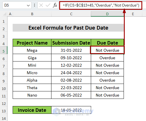
  
  Regards
  Abrar-ur-Rahman Niloy
  ExcelDemy
S M Dec 5, 2024 at 8:52 PM

How would I make this work for something that is not currently overdue, but was received late?
For example, I have reports that were due 06/21/2024 but were turned in 06/24/2024. They are not currently overdue, so the function with (Today) isn’t doing anything. But I want to flag the ones that were received late because I need to give metrics on how often we go over the due dates.

This article was very helpful and informative by the way, not quite what I needed in this specific instance but I will definitely be using this to notify me of overdue status for some of my other workbooks!
- Reply
  Shamima Sultana Dec 6, 2024 at 11:59 AM
  
  Hello SM,
  
  To flag reports that were received late but are not currently overdue, you can adjust the formula to check if the report was turned in later than the due date. You can compare the actual received date with the due date and flag it if the received date is later. Here’s an example of how you can modify your formula:
  
  Assume column A contains the due date and column B contains the received date:
  =IF(B2>A2, “Late”, “On Time”)
  
  This formula will flag the reports as “Late” if the received date (B2) is after the due date (A2). You can also add conditional formatting to highlight these “Late” entries.
  
  For metrics on how often you go over due dates, you can count how many reports are flagged as “Late” using a COUNTIF function:
  =COUNTIF(C2:C100, “Late”)
  
  This will give you a count of all reports that were received late.
  
  I’m glad the article was helpful, and I hope this solution better suits your needs for tracking late submissions! Let me know if you need further assistance with this adjustment.
  
  Regards
  ExcelDemy

How to Use Formula for Past Due Date in Excel (3 Methods)

How to Use a Formula for Past Due Date in Excel: 3 Ways

Method 1 – Using the Excel TODAY Function in Conditional Formatting for Past Due Date

Method 2 – Applying Excel IF and ISBLANK Functions for Past Due Date

Method 3 – Using Excel Combined Functions for Past Due Date

Practice Section

Related Articles

Leave a reply Cancel reply