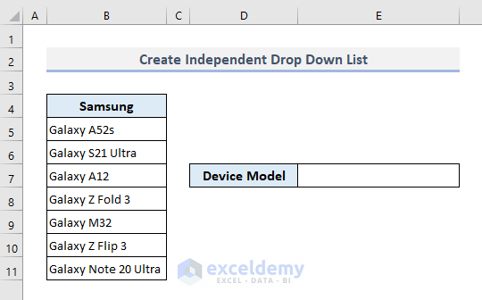
Example 1 – Create an Independent Drop-Down List in Excel
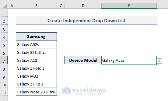
We have a list of popular Samsung smartphones. We’ll make a drop-down list in Cell E7 from where you can select any smartphone model listed in the chart.
Steps:
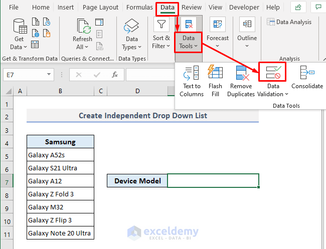
- Select the output Cell E7.
- Under the Data ribbon, select the Data Validation command from the Data Tools drop-down.
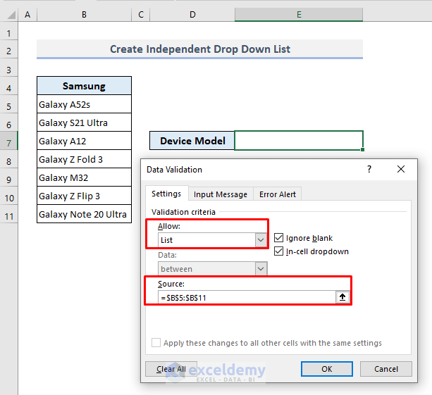
- In the Allow box, choose List from the options.
- Click on the Source box and select the range of cells (B5:B11) containing the model names of the smartphones.
- Press OK.
- Click on the drop-down button in Cell E7, and you’ll find the list of Samsung smartphones that are present in the table.
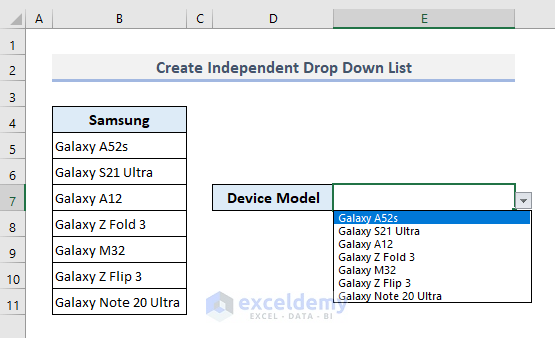
- Select any smartphone model and use it later as any other input data in a formula.
Read More: How to Create Drop Down List with Filter in Excel
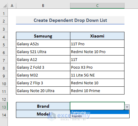
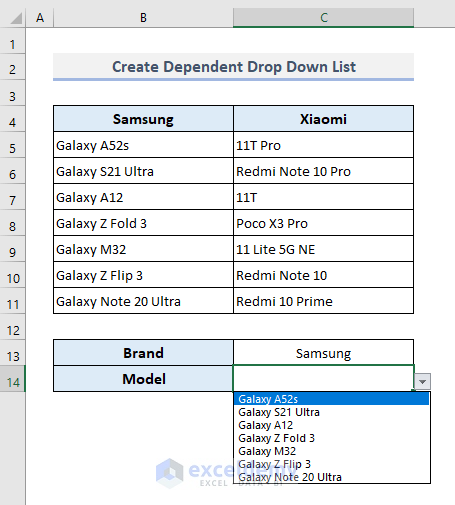
Example 2 – Create a Dependent Drop-Down List in Excel
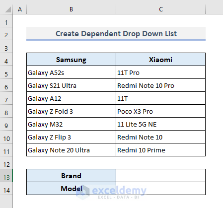
We have two columns containing smartphone models of two different renowned brands.
In Cell C13, we’ll create an independent drop-down list for the brand types. We’ll then make a dependent drop-down list in Cell C14 where smartphone models will be shown in a list based on the selected brand from the previous drop-down list.
Steps:
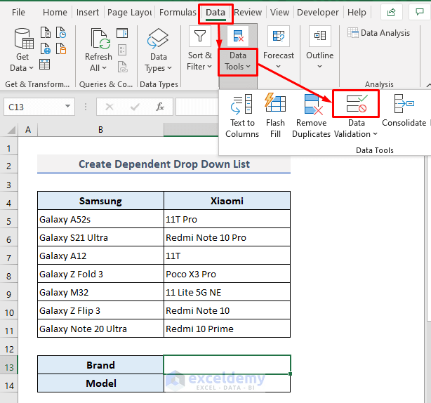
- Select Cell C13.
- Under the Data tab, choose the Data Validation command from the Data Tools drop-down.
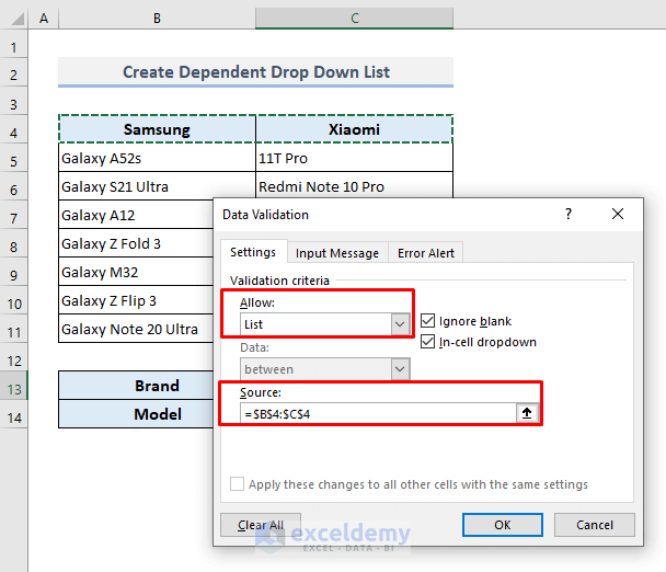
- In the Allow box, select List from the options.
- In the Source box, put the range of cells (B4:C4) containing the brand names of the smartphones.
- Press OK.
We’ve created an independent drop-down list for the smartphone brands in Cell C13.
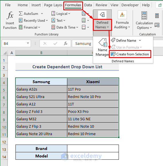
- Select the entire table or the range of cells B4:C11.
- Under the Formulas ribbon, choose the Custom from Selection command from the Defined Names drop-down.
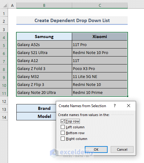
- Put a mark on the first option ‘Top row’ only and leave other options unmarked.
- Press OK.
We created two named ranges for two different smartphone brands with their corresponding models.
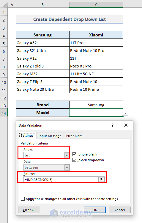
- Select cell C14.
- Open the Data Validation box again.
- Choose List in the Allow box.
- In the Source box, use the following formula:
=INDIRECT($C$13)- Press OK.
By using the INDIRECT function here, we’ve mentioned the cell reference of C13. The function will store the smartphone models in arrays for two different brands.
- Select a smartphone brand from the independent drop-down in Cell C13 and then click on the dependent drop-down button in Cell C14, and you’ll find all the smartphone models of the selected brand.
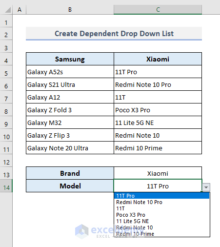
- Alter the smartphone brand, and you’ll find the corresponding smartphone models only, as shown in the screenshot below.
Read More: How to Create a Drop Down List with Unique Values in Excel
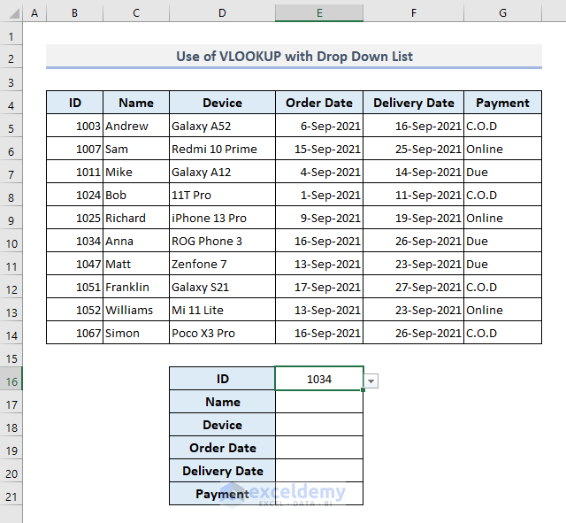
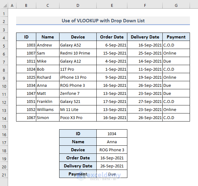
An Example of Using a Drop-Down List in Excel
Our dataset represents several order IDs for smartphone devices with the corresponding details. An independent drop-down list in Cell E15 has been created containing a list of order IDs. We’ll do is embed a formula in Cell E17 and extract all the available data for an order ID selected from the drop-down list.
Steps:
- Select the output Cell E17 and enter the following formula:
=TRANSPOSE(VLOOKUP(E16,B5:G14,{2,3,4,5,6},FALSE))- Press Enter.
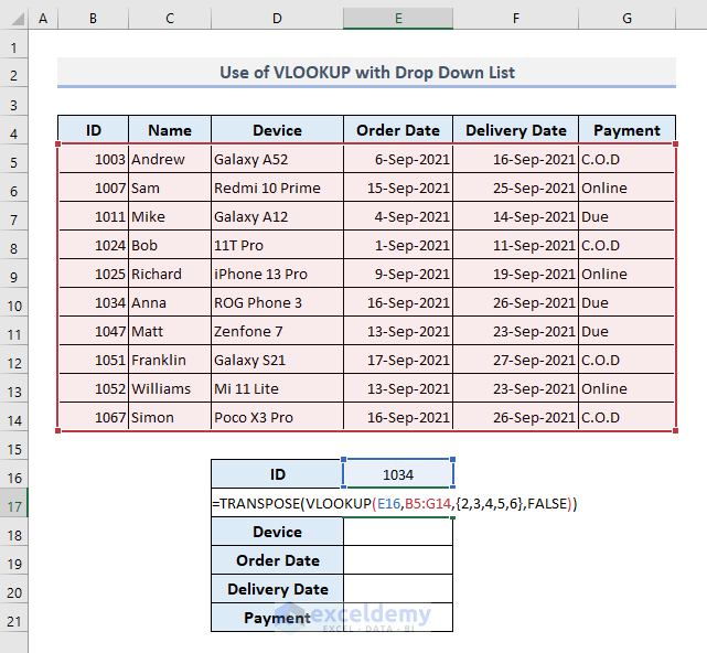
You’ll see all corresponding details for the selected order ID as displayed in the following screenshot.
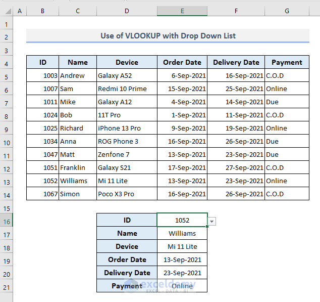
- Choose another order ID from the drop-down list.
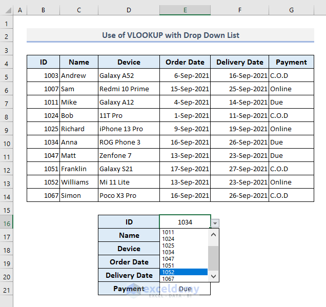
The output data will be updated.
Download the Practice Workbook
Create Drop Down List in Excel: Knowledge Hub
- Excel Data Validation Drop-Down List
- Create a Drop Down List from Another Sheet
- Create a Drop Down List with Unique Values
- Create Excel Drop Down List from Table
- Create Excel Drop Down List with Color
- Create a Searchable Drop Down List
- Creating a Drop Down Filter to Extract Data Based on Selection
- Create a Form with Drop Down List
- Fill Drop-Down List Cell in Excel with Color but with No Text
- Make Multiple Selection from Drop Down List
<< Go Back to Excel Drop-Down List | Data Validation in Excel | Learn Excel

