Method 1 – Use Simple Division to Calculate Ratio
- Select the cell where you want to calculate the ratio >> Write the following formula:
=C5/D5&":"&1- Press Enter >> Drag the Fill Handle to copy the formula in other cells.
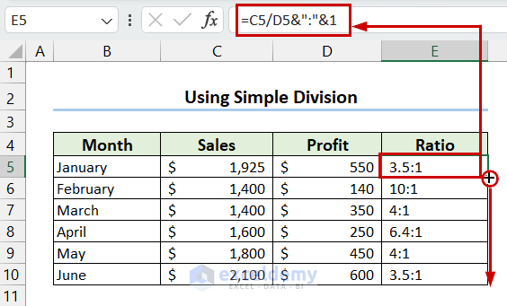
The value in cell C5 is divided by the value in cell D5, and the Ampersand (&) operator is used to join the result with “:” and 1.
Method 2 – Calculate the Ratio Using Excel GCD Function
- Select the cell where you want to calculate the ratio >> Write the following formula.
=C5/GCD(C5,D5)&":"&D5/GCD(C5,D5)- Press Enter >> Drag the Fill Handle to copy the formula in other cells.
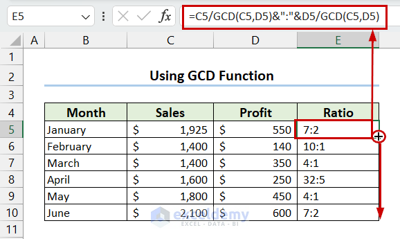
How Does the Formula Work?
- GCD(C5,D5): Here, the GCD function returns the greatest common divisor of the numbers in cells C5 and D5.
- C5/GCD(C5,D5): The value in cell C5 is divided by the GCD of C5 and D5 here.
- D5/GCD(C5,D5): Now, the value in cell D5 is divided by the GCD of C5 and D5.
- C5/GCD(C5,D5)&”:”&D5/GCD(C5,D5): Finally, the Ampersand (&) operator joins these 2 formulas with a Colon (:).
Method 3 – Use SUBSTITUTE And TEXT Functions to Calculate Ratio
- Select the cell where you want to calculate the ratio >> Write the following formula.
=SUBSTITUTE(TEXT(C5/D5,"####/####"),"/",":")- Press Enter >> Drag the Fill Handle to copy the formula in other cells.
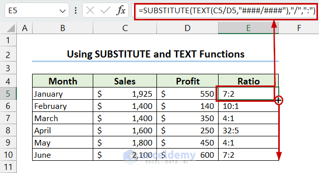
How Does the Formula Work?
- TEXT(C5/D5,”####/####”): The TEXT function returns the result in the desired format.
- SUBSTITUTE(TEXT(C5/D5,”####/####”),”/”,”:”): Now, the SUBSTITUTE function replaces Slash (/) with a Colon (:).
Method 4 – Apply the ROUND Function to Calculate the Ratio
- Select the cell where you want to calculate the ratio >> Write the following formula.
=ROUND(C5/D5,2)&":"&1- Press Enter >> Drag the Fill Handle down to copy the formula in other cells.
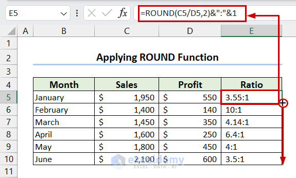
How Does the Formula Work?
- ROUND(C5/D5,2): Here, the ROUND function rounds the result to the given number of decimal places, which in this case is 2.
- ROUND(C5/D5,2)&”:”&1: Finally, the Ampersand (&) operator joins the result with a Colon (:) and 1.
How to Calculate Ratio Percentage in Excel
- Select the cell where you want to calculate the ratio percentage >> Write the following formula.
=C5/D5- Press Enter >> Drag the Fill Handle to copy the formula in other cells.
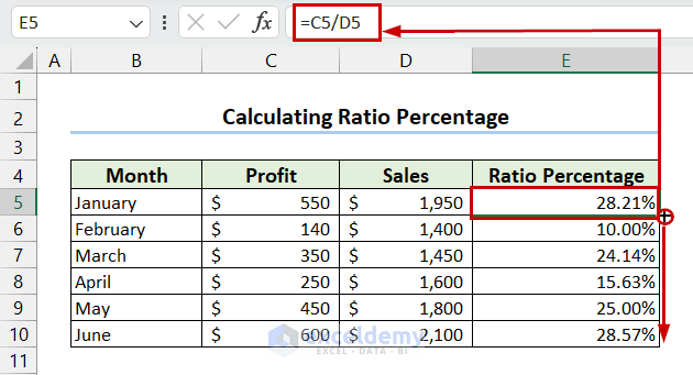
Note: For this method, you must select the cell format as Percentage.
Things to Remember
- As Excel does not provide a function for calculating ratios, you have to use functions according to your need to calculate Ratio in Excel.
- The second number can not be zero. Otherwise, it will return an error.
Frequently Asked Questions
1. What Is the Formula for the Ratio of 2 Numbers?
If the numbers are considered as x and y then the formula for the ratio will be x/y.
2. How to Calculate the Ratio of 3 Numbers?
You can use the GCD function to calculate the ratio of 3 numbers.
Download Practice Workbook
You can download the practice workbook from here.
Ratio in Excel: Knowledge Hub
<< Go Back to How to Calculate in Excel | Learn Excel
Get FREE Advanced Excel Exercises with Solutions!
