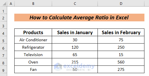
The sample Dataset showcases Products, Sales in January, and in February.
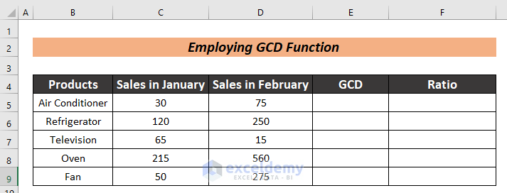
Method 1 – Using the GCD Function to Calculate the Average Ratio
Steps:
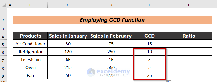
- Insert two additional columns: GCD and Ratio.
- To find the GCD, enter the following formula in a cell. Here, E5.
=GCD(C5,D5)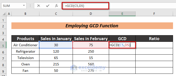
- Press ENTER.
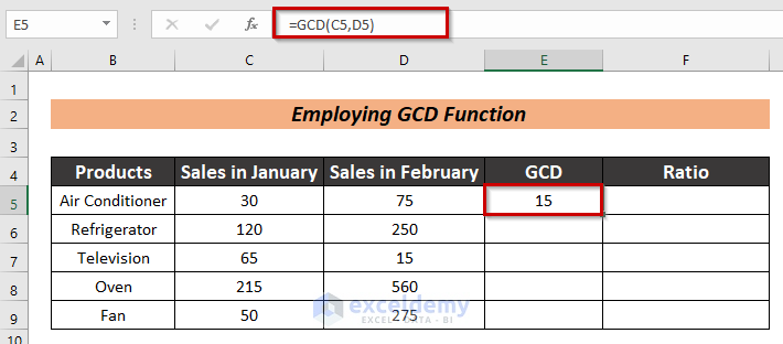
- Drag down the Fill Handle to see the result in the rest of the cells.
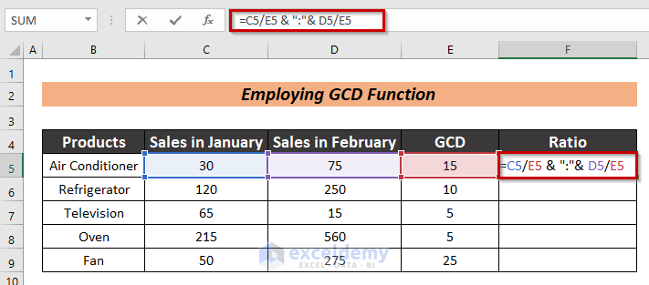
- Use the following formula to find the Ratio:
=C5/E5 & ":"& D5/E5Values in C5 and D5 are divided by the greatest common divisor and presented as a ratio (values are concatenated using a colon).
- Press ENTER to see the Ratio.
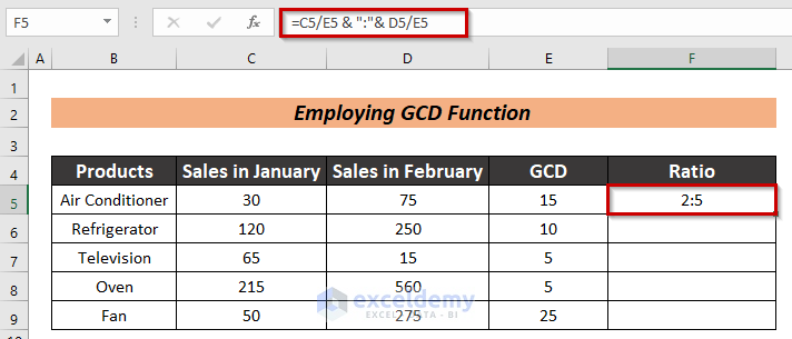
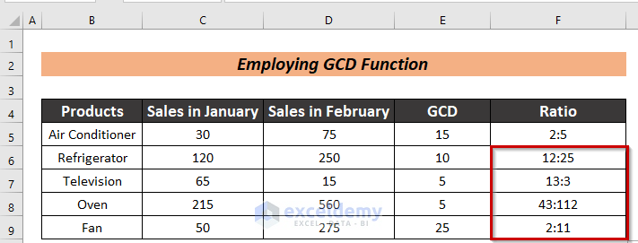
- Drag down the Fill Handle to see the result in the rest of the cells.
To calculate the average:
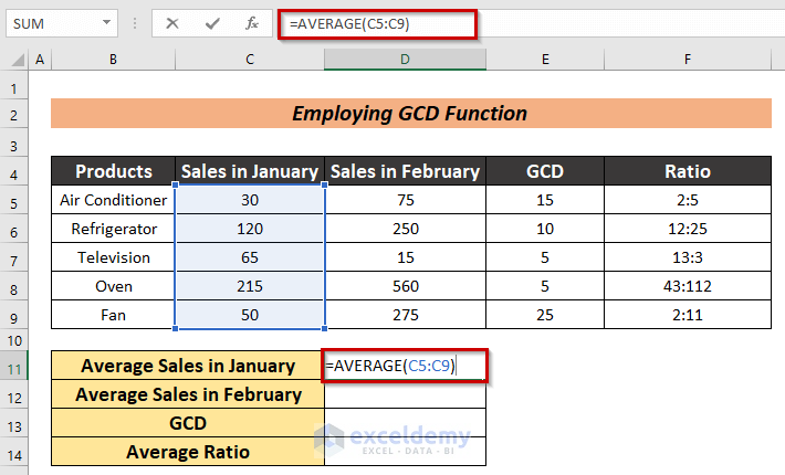
- Use the following formula to get the Average Sales in January:
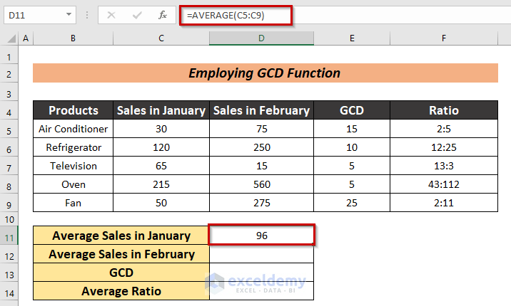
=AVERAGE(C5:C9)
- Press ENTER to see the Average Sales in January.
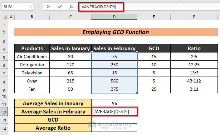
- Use the same formula to find the Average Sales in February:
=AVERAGE(D5:D9)
- Press ENTER.

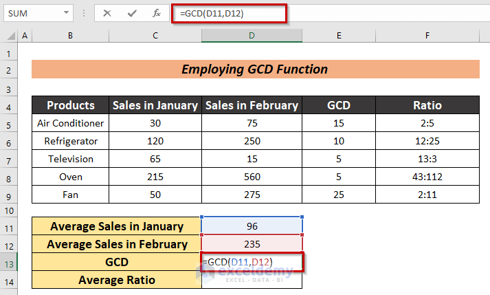
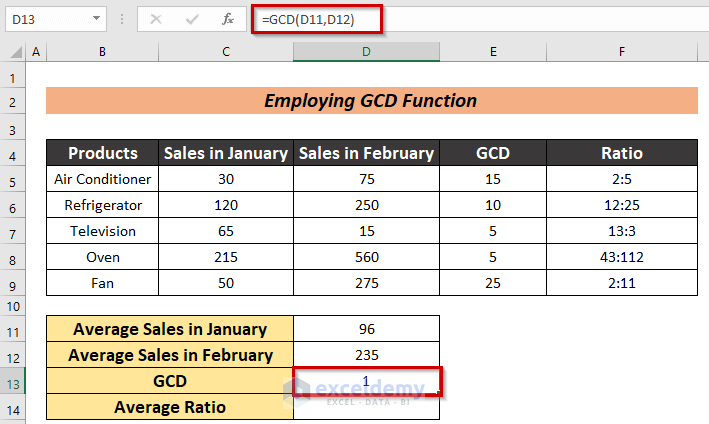
- To find the Greatest Common Divisor between the Average Sales in January and the Average Sales in February use the following equation:
=GCD(D11,D12)
- Press ENTER.
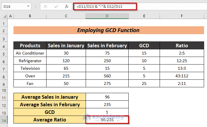
- Use the formula below to find the Average Ratio:
=D11/D13 & ":"& D12/D13
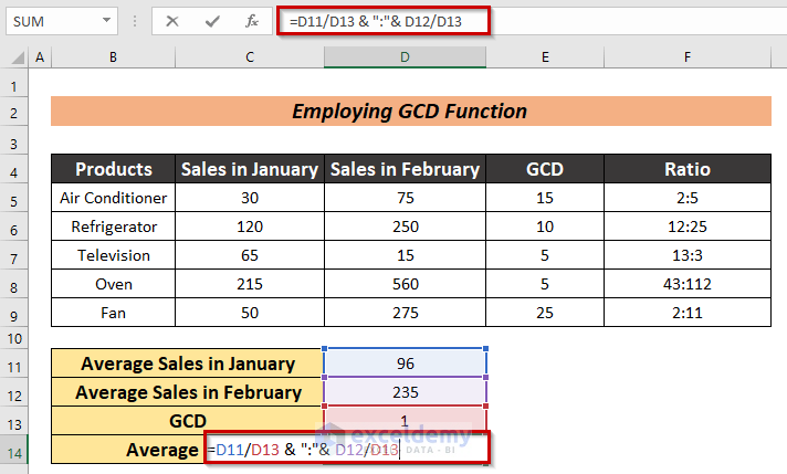
- Press ENTER.
Read More: How to Calculate Ratio of 3 Numbers in Excel
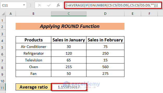
Method 2 – Combining the ISNUMBER, IF and AVERAGE Functions
Steps:
- Select a cell to enter the formula. Here, C11.
=AVERAGE(IF(ISNUMBER(C5:C9/D5:D9),C5:C9/D5:D9,""))
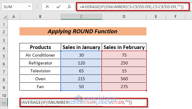
- Press ENTER to see the Average Ratio.
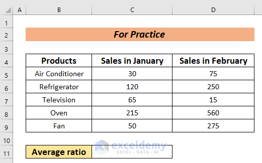
Practice Section
Practice here.
Download Practice Workbook
Related Articles
- How to Calculate Male Female Ratio in Excel
- How to Calculate Sortino Ratio in Excel
- How to Calculate Sharpe Ratio in Excel
- How to Calculate Odds Ratio in Excel
- How to Calculate Compa Ratio in Excel
<< Go Back to Ratio in Excel | Calculate in Excel | Learn Excel
Get FREE Advanced Excel Exercises with Solutions!
