What Is the Sortino Ratio?
The Sortino ratio is a risk-adjustment statistics metric used to calculate the return from a certain investment for a given level of negative risk. It is a refined version of the more widely known Sharpe ratio. The Sharpe ratio considers total price deviation in the calculation, while the Sortino ratio considers a downside deviation while calculating.
The basic formula to calculate the Sortino ratio is:
=(Rp–Rf)/σd- Rp is the portfolio’s Expected Return or Actual Return.
- Rf is the portfolio’s Minimum Acceptable Return (MAR)/Risk-free rate of return.
- σd is the Downside Deviation or Standard Deviation of negative asset return.
How to Calculate the Sortino Ratio in Excel: 2 Methods
Method 1 – Calculate the Sortino Ratio Using Excel Formulas
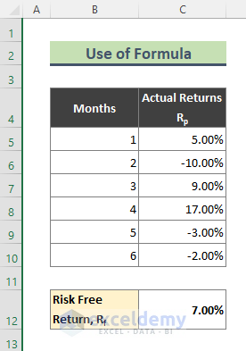
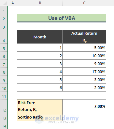
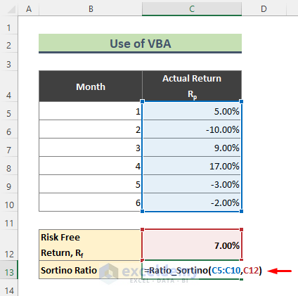
We have the average return percentage of a certain company for 6 months. The risk-free return of the portfolio is 7%.
Steps:
- Calculate the Excess Return with the following formula in Cell D5.
=C5-$C$13- Press Enter.
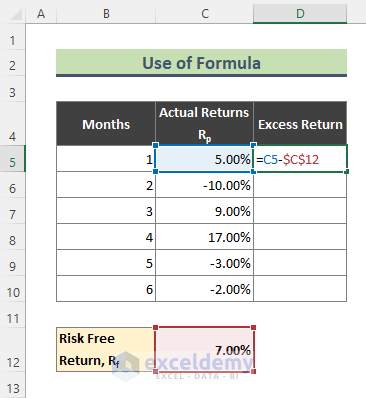
- Use the Fill Handle (+) tool to get the return for the rest of the values.
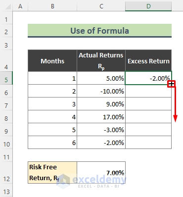
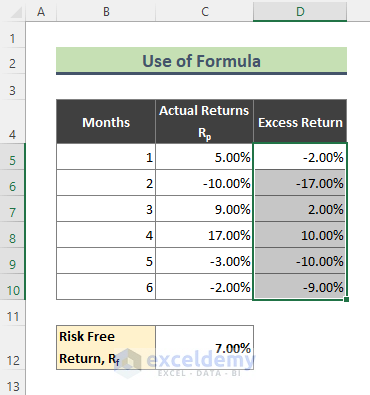
- Here’s the result.
- We will separate only Negative Excess Returns with the following formula in E5, then using AutoFill through the column.
=IF(D5<0,D5,0)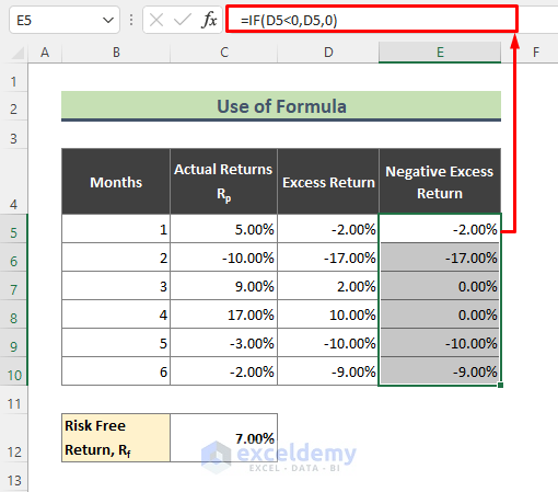
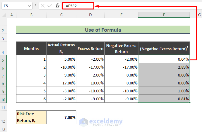
- Use the following formula to calculate the square of Negative Excess Returns.
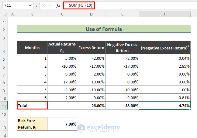
- Use the SUM function for the total of Excess Returns.
- We also calculated the total of the square of Negative Excess Return values using the SUM formula.
- Calculate the average of the Excess Return using the following formula:
=D11/6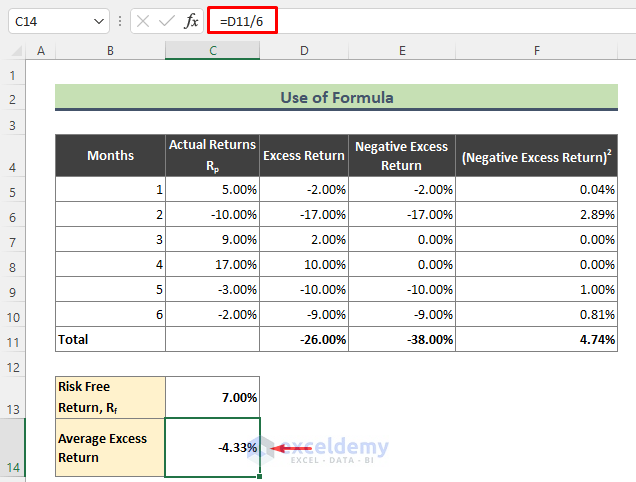
The formula to calculate the Downside Risk is:
=√(∑(Square of Negative Excess Returns)/No. of months)- Use this formula to calculate Downward Risk:
=SQRT(F11/6)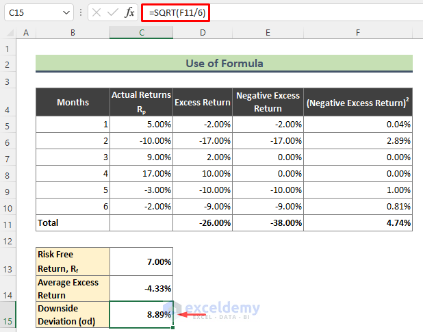
- To calculate the Sortino ratio, divide Average Excess Return by Downside Risk.
=C14/C15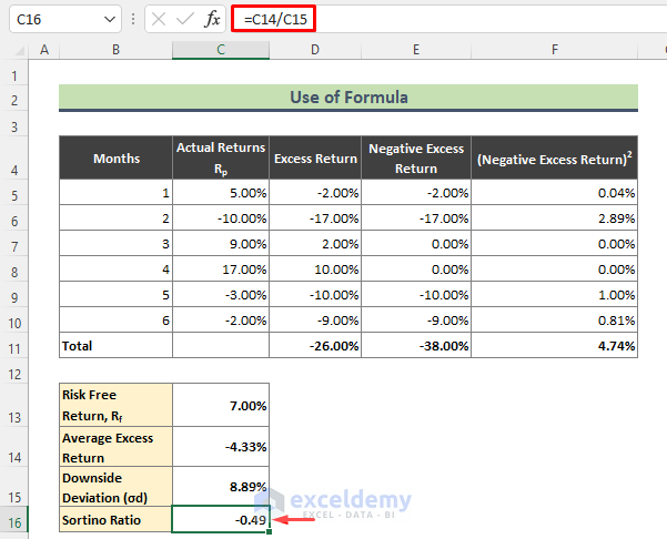
Note:
If you want to calculate the Sortino ratio against the Actual Return of a random month, follow these steps:
- After calculating the Downside Risk following the steps above, subtract the Risk-Free Return from the specific Actual Return.
- To calculate the Sortino ratio for the Average Return of Cell C7, use the below formula:
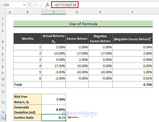
=(C7-C13)/C14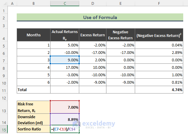
- You can calculate the Sortino ratio for any other Actual Return and thus compare which investment is safe.
Read More: How to Calculate Sharpe Ratio in Excel
Method 2 – Excel VBA to Calculate the Sortino Ratio
We will use the same dataset that was used in Method 1.
Steps:
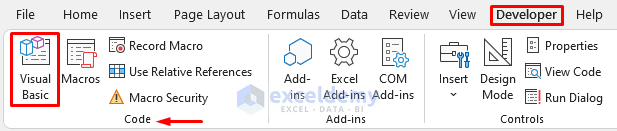
- From the Ribbon, go to the Developer tab.
- Select Visual Basic.
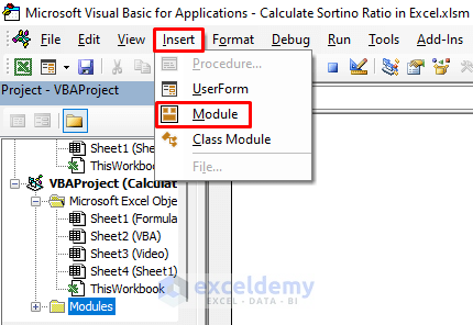
- The VBA window will appear.
- Go to the Insert option.
- Select a new Module.
- Use the following code in the newly inserted Module.
Function Ratio_Sortino(returns As Range, MAR As Variant) As Variant
Dim x As Integer
Dim y As Integer
Dim RetAvg As Double
Dim m2 As Double
Dim dev As Double
x = returns.Rows.Count
RetAvg = WorksheetFunction.Average(returns)
moment2d = 0
For y = 1 To x
If returns(y) - MAR < 0 Then
m2 = m2 + ((returns(y) - MAR) ^ 2)
End If
Next
dev = Sqr(m2 / x)
If dev > 0 Then
Ratio_Sortino = (RetAvg - MAR) / dev
Else
Ratio_Sortino = "undefined"
End If
End Function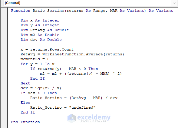
- Use this formula in Cell C13 and hit Enter.
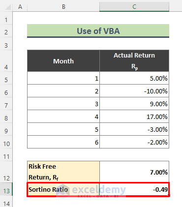
- We will get the Sortino ratio for the above data.
Read More: How to Calculate Ratio of 3 Numbers in Excel
Observations from Calculating the Sortino Ratio
- By calculating the Sortino ratio for a specific portfolio’s Actual Return, you can check the return on investment.
- By comparing the Sortino ratio of certain actual returns, you can check which investment is safer to pursue.
- The Sortino ratio is really helpful to retail investors as it helps them to make the right decision about any investment.
Download the Practice Workbook
Related Articles
- How to Calculate Average Ratio in Excel
- How to Calculate Male Female Ratio in Excel
- How to Calculate Odds Ratio in Excel
- How to Calculate Compa Ratio in Excel
<< Go Back to Ratio in Excel | Calculate in Excel | Learn Excel
Get FREE Advanced Excel Exercises with Solutions!
