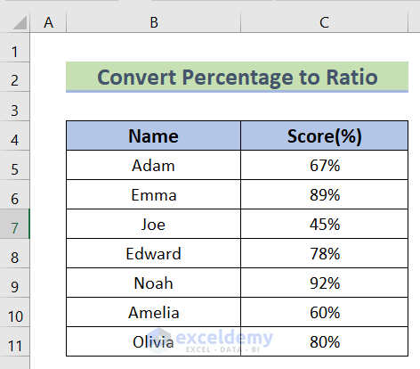
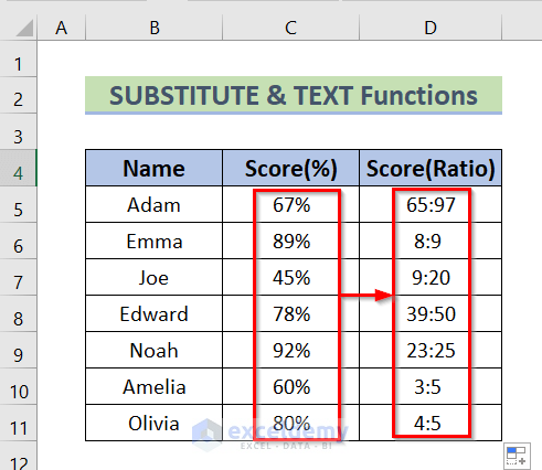
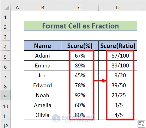
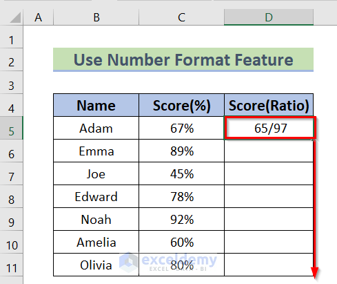
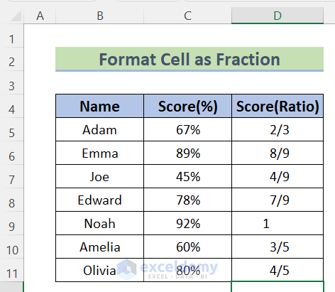
We have the following dataset containing the mark sheets of some students. Scores are given in percentages. We will convert these percentage values to Ratios.
Method 1 – Using a Combination of Excel SUBSTITUTE and TEXT Functions
Steps:
- In cell D5, insert the following formula.
=SUBSTITUTE(TEXT(C5,"?/??"),"/",":")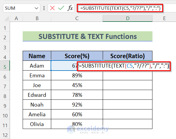
Formula Breakdown
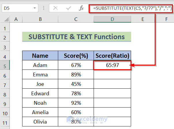
- TEXT(C5,”?/??”)—–> The TEXT function will format the selected value using a divider.
- Output: “65/97”
- SUBSTITUTE(TEXT(C5,”?/??”),”/”,”:”)—-> becomes
- SUBSTITUTE(“65/97″,”/”,”:”)—–> The SUBSTITUTE function will replace the divider with
- Output: 65:97
- SUBSTITUTE(“65/97″,”/”,”:”)—–> The SUBSTITUTE function will replace the divider with
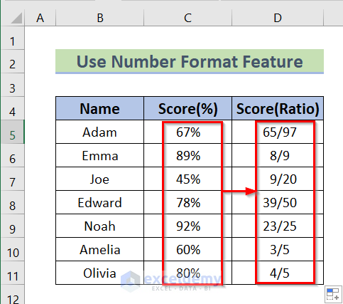
- Press Enter to get the ratio.
- Drag down the Fill Handle tool to AutoFill the formula for the rest of the cells.
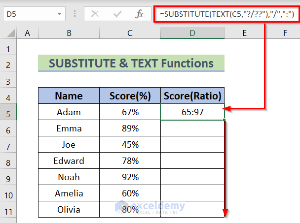
- The values are now converted into a ratio from a percentage.
Read More: How to Calculate Ratio Percentage in Excel
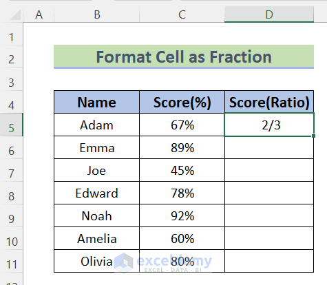
Method 2 – Formatting the Cell as a Fraction
Steps:
- In cell D5, insert the following formula.
=C5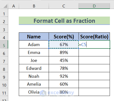
- Press Enter to get the value in the resultant cell.
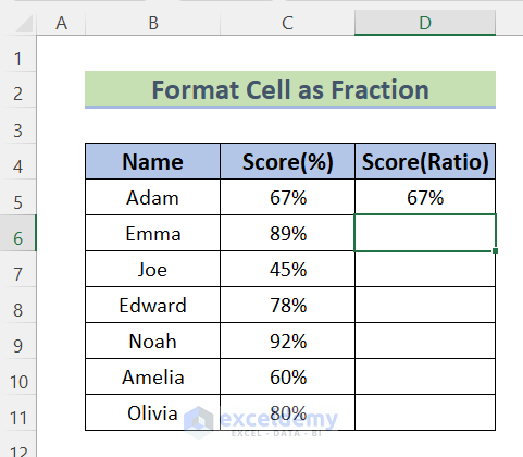
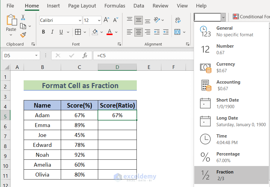
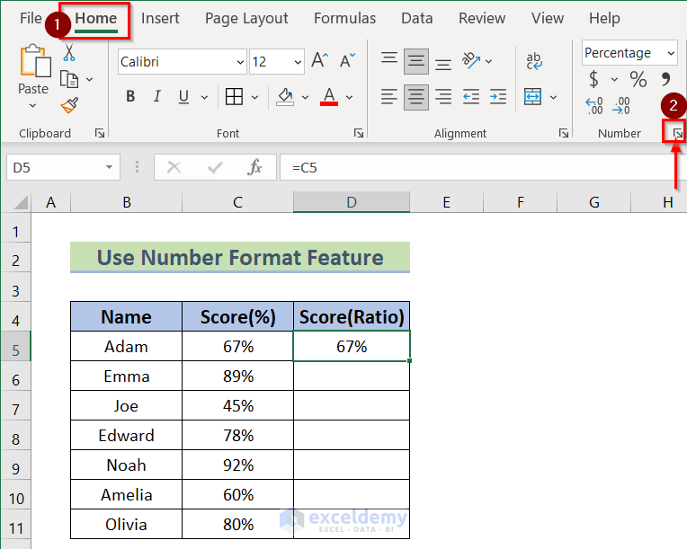
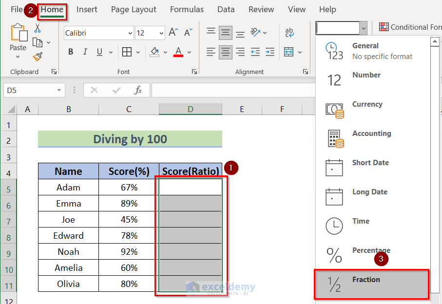
- Select cell D5.
- Open the Home tab, and from Number Format, select Fraction
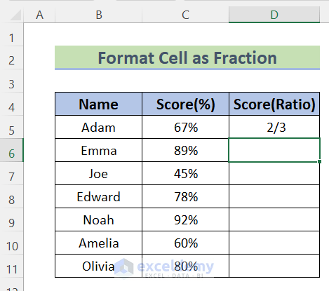
- This’ll convert the percentage to a ratio.
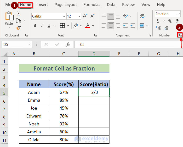
- To get a more precise value, you can use the Format Cell: Click on the Number Format icon from the Number group of the Home.
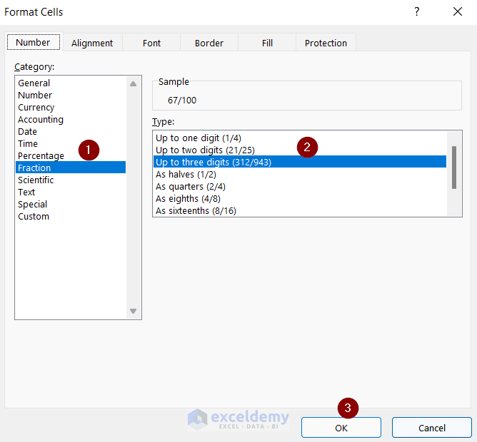
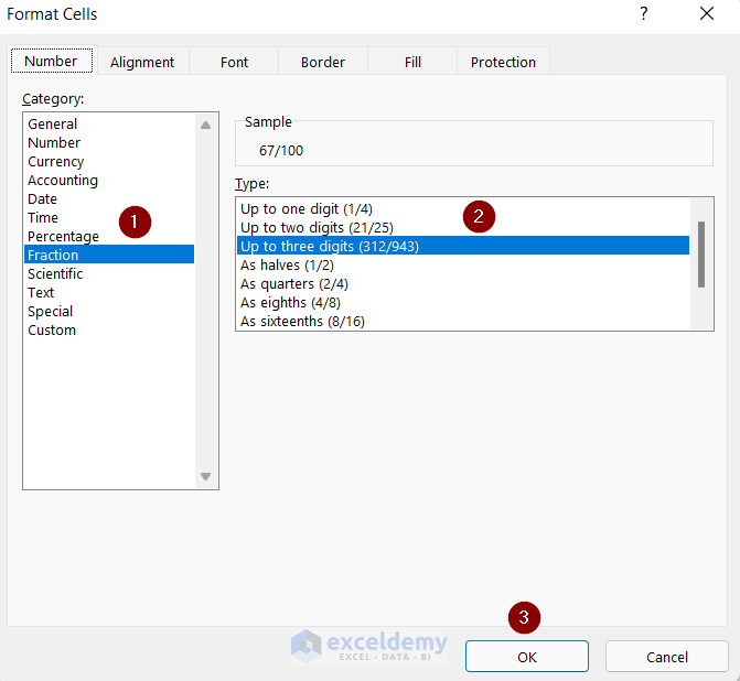
- In the Format Cells dialog box, click on Fraction from the Category box.
- Select Up to three digits (312/943).
- Press OK.
- Drag down the Fill Handle tool to AutoFill the formula with the Format.
All the values are converted into ratios from percentages.
Similar Readings
Method 3 – Using the Custom Format Feature
Steps:
- In cell D5, insert the following formula.
<span style="font-size: 14pt;">=C5</span>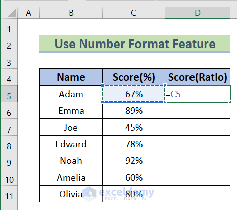
- Click on the Number Format icon from the Number section of the Home ribbon.
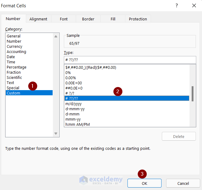
- In the Format Cells dialog box, click on Custom from the Category box.
- Choose #??/?? from the Type box.
- Press OK.
- Drag down the Fill Handle to AutoFill the rest of the cells.
- The values are now converted to ratios from percentages.
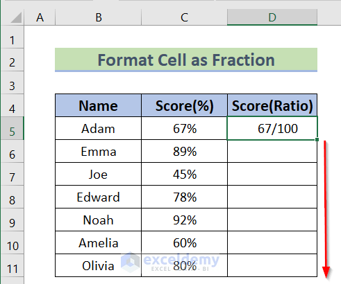
Method 4 – Dividing a Percentage Value by 100 to Get a Ratio
Steps:
- Select the cells you want to put the resultant ratio values. We have selected Cell D5:D11.
- Click on Home, then from Number group, select Fraction.
- In cell D5, insert the following formula.
<span style="font-size: 14pt;">=67/100</span>
- Press Enter to get the ratio from the percentage.
- Repeat for other cells in the column.
If the ratio is close to 1, the resultant ratio shows as 1:1. We can customize the Fraction format as Up to three digits.
- Select cells D5:D11.
- Right-click on and select Format Cells
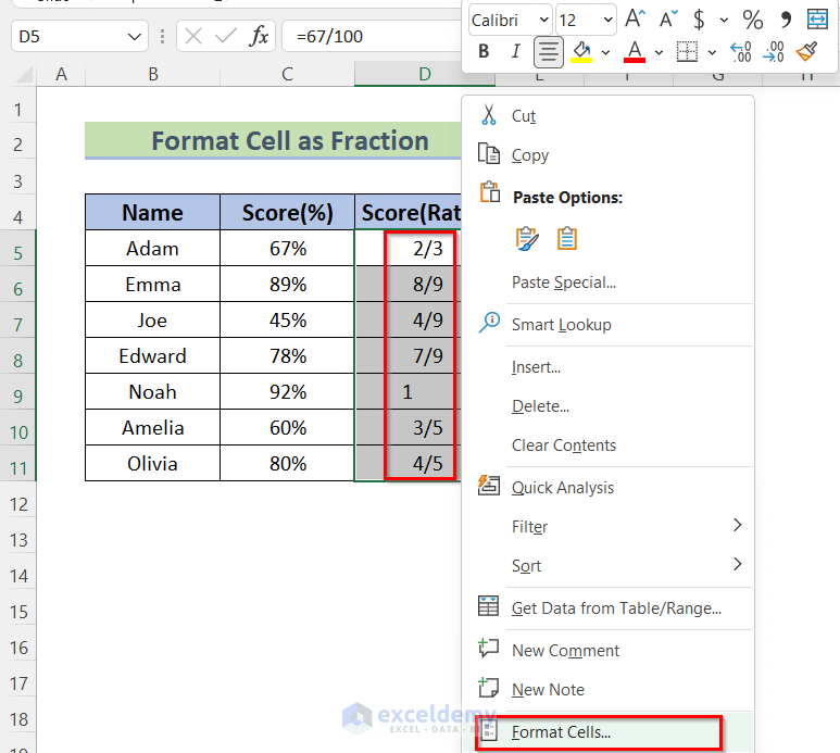
- From the Number format, get some custom Fraction formats in the Type box. Choose Up to three digits (312/943).
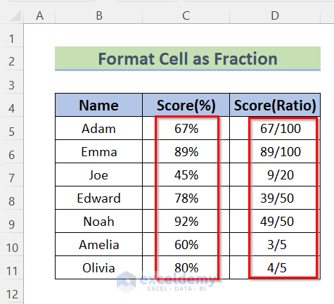
- Press OK.
- The values are now converted to ratios.
Download the Practice Workbook
Related Articles
- How to Graph Ratios in Excel
- How to Use Interest Coverage Ratio Formula in Excel
- Debt Service Coverage Ratio Formula in Excel
- How to Do Ratio Analysis in Excel Sheet Format
- How to Convert Ratio to Decimal in Excel
<< Go Back to Ratio in Excel | Calculate in Excel | Learn Excel
Get FREE Advanced Excel Exercises with Solutions!
