How to Use Interest Coverage Ratio Formula in Excel (2 Easy Methods)

If you are looking for some special tricks to use the interest coverage ratio formula in Excel, you’ve come to the right place. There are numerous ways to use the interest coverage ratio formula in Microsoft Excel. This article will discuss two methods to use the interest coverage ratio formula in Excel. Let’s follow the complete guide to learn all of this.

What Is Interest Coverage Ratio?

The interest coverage ratio measures an entity’s ability, so that, interest payments on its debts can be made when they come due. An increasing ratio indicates a company’s ability to meet its interest expense obligations comfortably. In determining the company’s liquidity, lenders, such as banks and investors, use this ratio.

Types of Interest Coverage Ratio

There are two types of interest coverage ratios. The first type is obtained by dividing EBIT by Interest Expenses. The second type is obtained by dividing EBITDA by Interest Expenses. The Formulas are given below:

Interest Coverage Expense= (EBIT)/Interest Expense
Interest Coverage Expense= (EBITDA)/ Interest Expense

Here, EBIT means Earnings before interest and tax. And EBITDA means earnings before interest, tax, depreciation, and amortization.

Significance of Interest Coverage Ratio

An interest coverage ratio of 1 indicates that the company is in a risky condition. Financial institutions will never lend to these types of companies since they are in a poor financial situation.
When a company pays interest on its debt, the interest coverage ratio must be greater than 1. If the interest coverage ratio is between 1 and 1.5, the company is in red alert condition.

Simple Example of Interest Coverage Ratio

Here, we are going to show the simple calculation of interest coverage. The following image shows a company’s net operating profit, interest income, and interest expense for 2020.

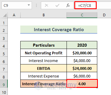
In order to use the interest coverage ratio formula of the company, we need to add net profiting income with interest income. Then divide it by interest expense. For the above data, we have to do the following calculation:

Interest Coverage Ratio=($20000+$4000)/$6000

As a result, we will get an interest coverage ratio of 4. This value means the above company’s profits are able to cover the interest 4 times.

How to Use Interest Coverage Ratio Formula in Excel: 2 Suitable Ways

We will use two effective and tricky methods to use the interest coverage ratio formula in Excel. This section provides extensive details on the two methods. You should learn and apply all of these, as they improve your thinking capability and Excel knowledge.

1. Using EBITDA Method

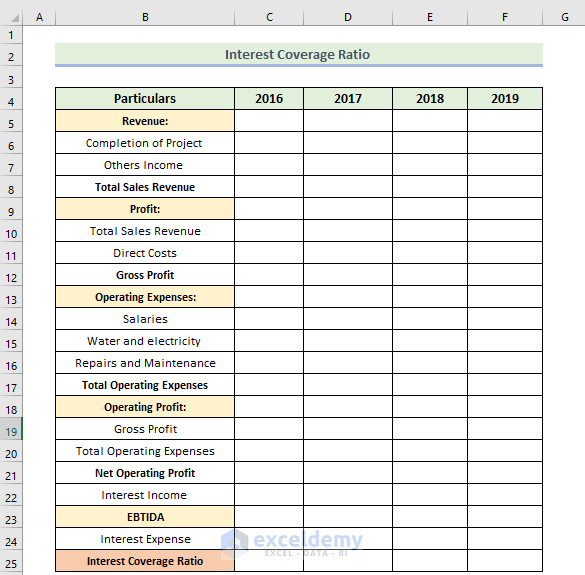
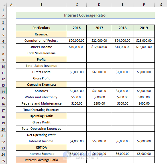
Here, we will demonstrate how to calculate the interest coverage ratio in Excel. Let us first introduce you to our Excel dataset so that you are able to understand what we are trying to accomplish with this article. The dataset provides details of the expenses and income of a company over the last four years. Our goal now is to calculate the company’s interest coverage ratio over the last four years. Let’s walk through the steps to calculate the interest coverage ratio.

📌 Steps:

Firstly, enter the amount of money of the company in the Revenue, Operating Expenses, Interest Income, and Interest Expense section.

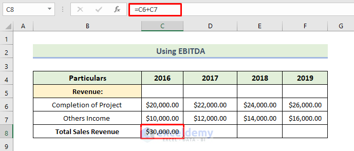
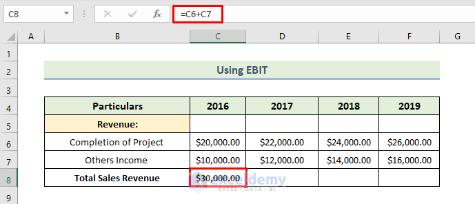
Next, we want to calculate the total sales revenue of the company. Therefore, we will use the following formula in the cell C8:

=C6+C7

Here, cell C6 is the income of the company by the completion of the project. Cell C7 is the company’s other income.

Press Enter.

Next, drag the Fill Handle icon to the right.
Therefore, you will obtain the company’s total sales revenue over the last four years.

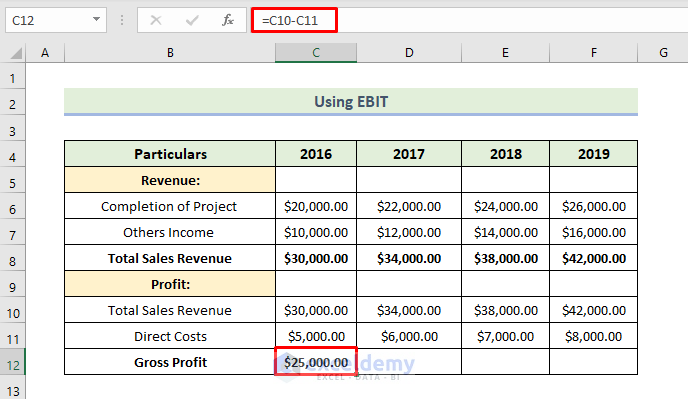
Next, we want to calculate gross profit. Therefore, we will use the following formula in the cell C12:

=C10-C11

Here, cell C10 is the amount of the company’s total sales revenue. Cell C11 is the direct cost of the company.

Press Enter.

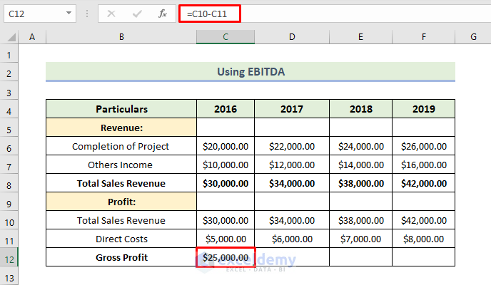
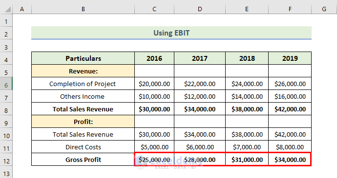
Next, drag the Fill Handle icon to the right.
Therefore, you will obtain the company’s gross profit over the last four years.

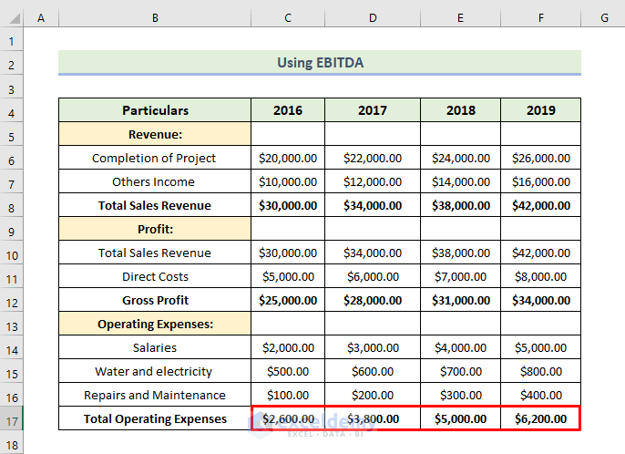
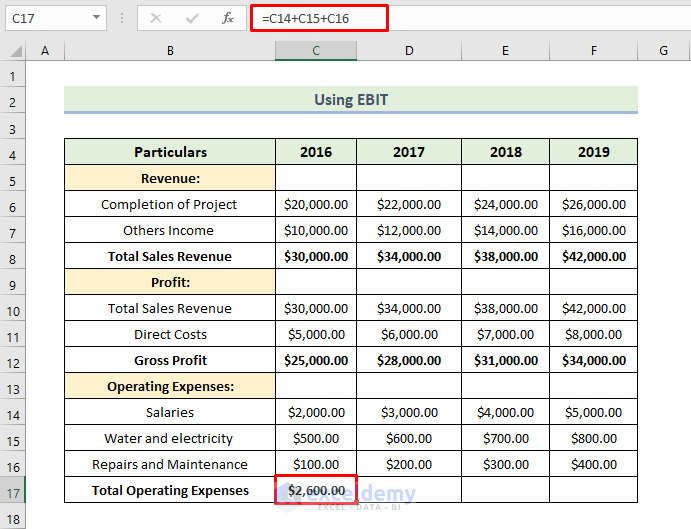
Next, we want to calculate the total operating expenses of the company. Therefore, we will use the following formula in cell C17:

=C14+C15+C16

Then press Enter.

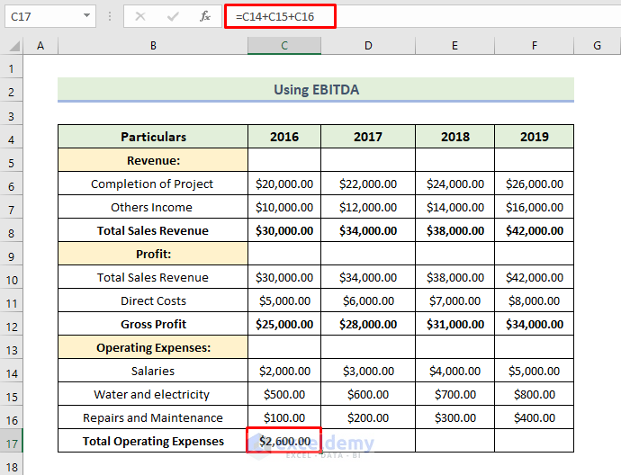
Next, drag the Fill Handle icon to the right.
Therefore, you will obtain the company’s total operating expenses over the last four years.

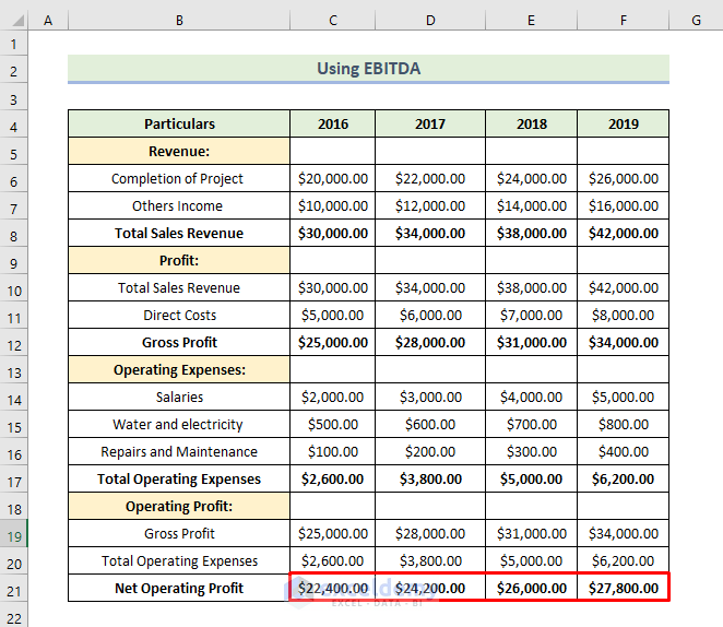
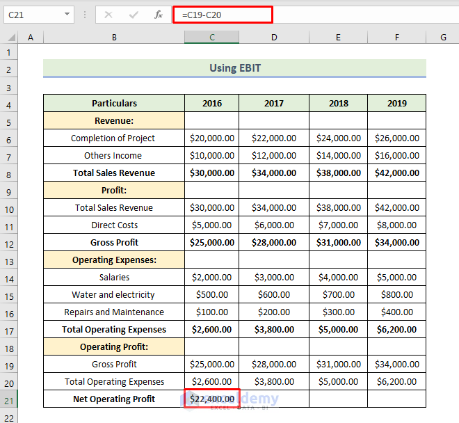
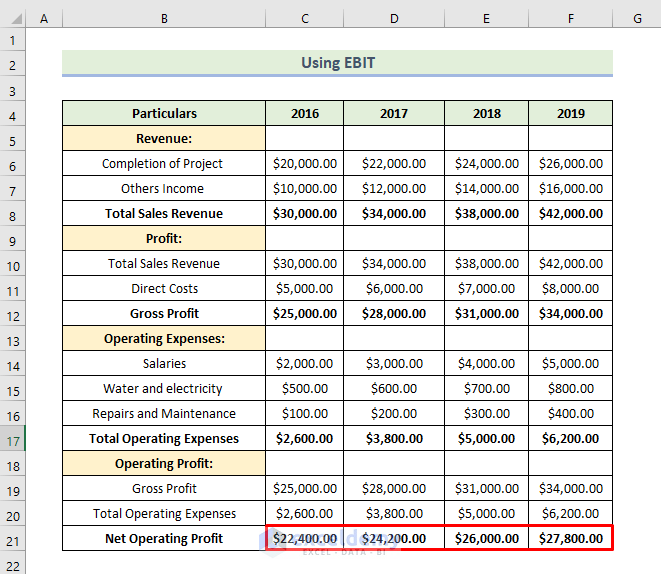
Next, we want to calculate the net operating profit of the company. Therefore, we will use the following formula in the cell C21:

=C19-C20

Here, cell C19 is the amount of the company’s gross profit. Cell C20 is the total operating expenses of the company.

Press Enter.

Next, drag the Fill Handle icon to the right.
Therefore, you will obtain the company’s net operating profit over the last four years

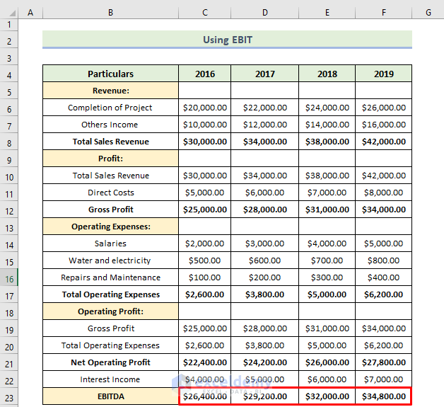
Next, we want to calculate the EBITDA of the company. Therefore, we will use the following formula in the cell C23:

=C21+C22

Here, cell C21 is the amount of the company’s net operating profit. Cell C22 is the interest income of the company.

Press Enter.

Next, drag the Fill Handle icon to the right.
Therefore, you will obtain the company’s EBITDA over the last four years

Next, we want to calculate the Interest Coverage Ratio of the company. Therefore, we will use the following formula in the cell C25:

=C23/C24

Here, cell C23 is the amount of the company’s EBITDA. Cell C24 is the interest expense of the company.

Press Enter.

Next, drag the Fill Handle icon to the right.
Therefore, you will obtain the company’s interest coverage ratio over the last four years

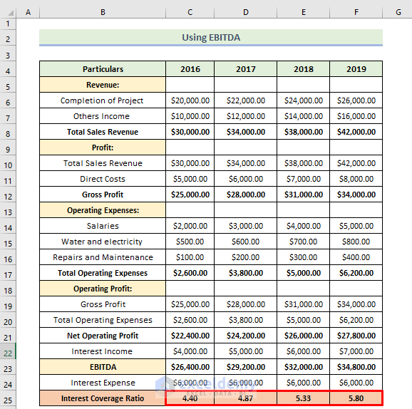
we will get an interest coverage ratio of 4.40 which means the above company’s profits are able to cover the interest 4.4 times. From the above calculation, we see that the interest coverage ratio increases every year. This is a good sign for the company. That means the company is in stable condition.

2. Utilizing EBIT Method

Here, we will use another method to calculate the interest coverage ratio of the company. In this method, the interest coverage ratio is obtained by dividing EBIT by Interest Expenses. Let’s walk through the steps to calculate the interest coverage ratio.

📌 Steps:

Firstly, enter the amount of money the company in the Revenue, Operating Expenses, interest income, and interest expense section.

Next, we will use the following formula in the cell C8:

=C6+C7

Here, cell C6 is the income of the company by the completion of the project. Cell C7 is the company’s other income.

Press Enter.

Next, drag the Fill Handle icon to the right.
Therefore, you will obtain the company’s total sales revenue over the last four years.

Next, we will use the following formula in the cell C12:

=C10-C11

Here, cell C10 is the amount of the company’s total sales revenue. Cell C11 is the direct cost of the company.

Then, press Enter.

Next, drag the Fill Handle icon to the right.
Therefore, you will obtain the company’s gross profit over the last four years.

Next, we want to calculate the total operating expenses of the company. Therefore, we will use the following formula in cell C17:

=C14+C15+C16

Then, press Enter

Next, drag the Fill Handle icon to the right.
Therefore, you will obtain the company’s total operating expenses over the last four years.

Next, we want to calculate the net operating profit of the company. Therefore, we will use the following formula in the cell C21:

=C19-C20

Here, cell C19 is the amount of the company’s gross profit. Cell C20 is the total operating expenses of the company.

Then, press Enter.

Next, drag the Fill Handle icon to the right.
Therefore, you will obtain the company’s net operating profit over the last four years

Next, we want to calculate the EBITDA of the company. Therefore, we will use the following formula in the cell C23:

=C21+C22

Here, cell C21 is the amount of the company’s net operating profit. Cell C22 is the interest income of the company.

Then, press Enter.

Next, drag the Fill Handle icon to the right.
Therefore, you will obtain the company’s EBITDA over the last four years

Next, we want to calculate the EBIT of the company. Therefore, we will use the following formula in the cell C27:

=C25-C26

Here, cell C25 is the amount of the company’s EBITDA. Cell C26 is the depreciation of the company.

Then, press Enter.

Next, drag the Fill Handle icon to the right.
Therefore, you will obtain the company’s EBIT over the last four years

Next, we want to calculate the Interest Coverage Ratio of the company. Therefore, we will use the following formula in the cell C29:

=C27/C28

Here, cell C27 is the amount of the company’s EBIT. Cell C28 is the interest expense of the company.

Then, press Enter.

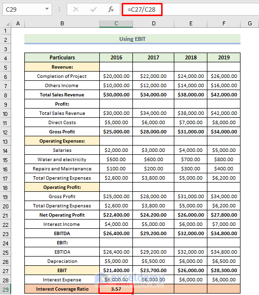
Next, drag the Fill Handle icon to the right.
Therefore, you will obtain the company’s interest coverage ratio over the last four years

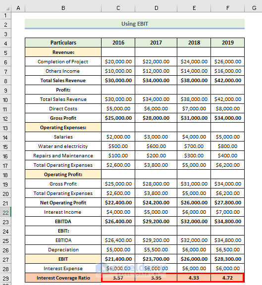
we will get an interest coverage ratio of 3.57 which means the above company’s profits are able to cover the interest 3.57 times. From the above calculation, we see that the interest coverage ratio increases every year. This is a good sign for the company. That means the company is in stable condition.

Download Practice Workbook

Interest Coverage Ratio.xlsx

Conclusion

That’s the end of today’s session. I strongly believe that from now you may calculate the interest coverage ratio in Excel. If you have any queries or recommendations, please share them in the comments section below. Keep learning new methods and keep growing!

<< Go Back to Ratio in Excel | Calculate in Excel | Learn Excel

Get FREE Advanced Excel Exercises with Solutions!