Understanding Ratios
- Ratios express the relative size between two or more numbers.
- The ratio is obtained by dividing one number (the antecedent) by another (the consequent).
- The general format of a ratio is a:b, where a and b can be integers, decimals, or fractions.
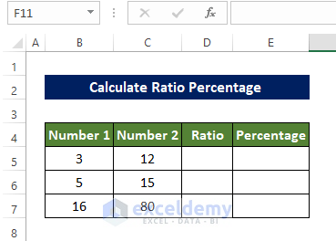
Dataset Overview
- Let’s use a dataset with two columns: Number 1 (in column B) and Number 2 (in column C).
- We want to calculate the ratio of Number 1 to Number 2 and express it as a percentage.
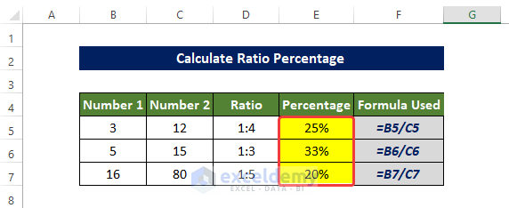
Method 1 – Using the GCD Function
- The GCD function finds the greatest common divisor between two numbers.
- We’ll use this value to calculate the ratio and percentage.
Step-by-Step Calculation
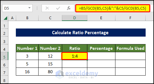
- In cell D5, enter the following formula:
=B5/GCD(B5,C5)&":"&C5/GCD(B5,C5)This formula calculates the ratio between cell B5 and C5 and displays it as a:b in cell D5.
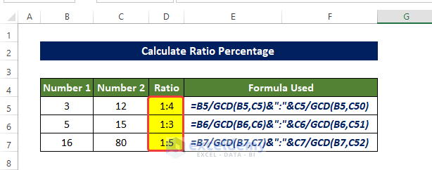
- Drag the Fill Handle down to cell D7 to fill the entire range (D5:D7) with ratios.
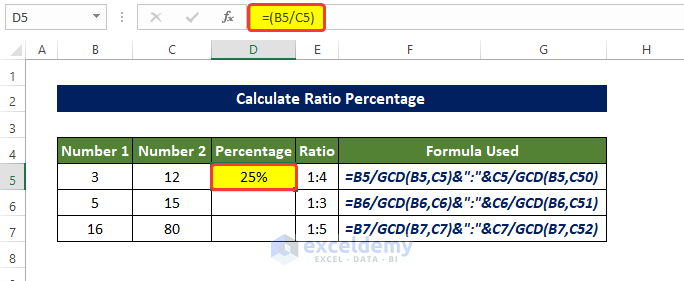
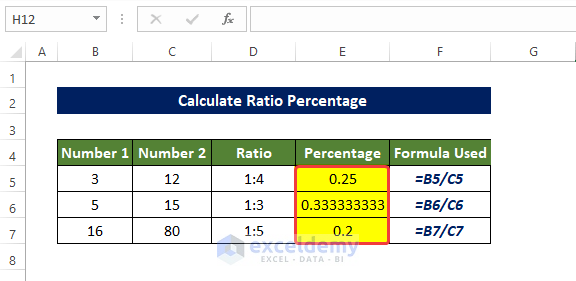
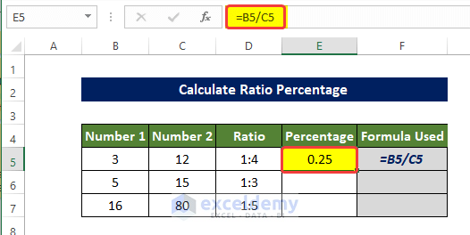
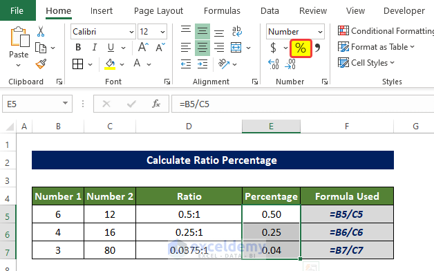
- In cell E5, enter the formula:
=B5/C5
This calculates the quotient of Number 1 divided by Number 2.
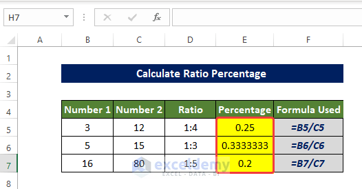
- Drag the Fill Handle down to cell E7 to fill the entire range (E5:E7) with quotient values.
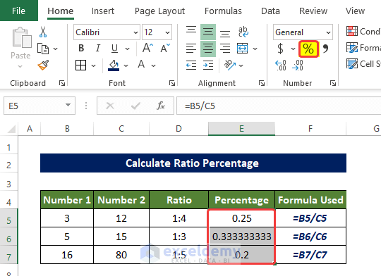
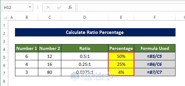
- Select the range E5:E7, go to the Home tab, and click the % (Percentage) sign in the Number group. This converts the quotient values to percentages.
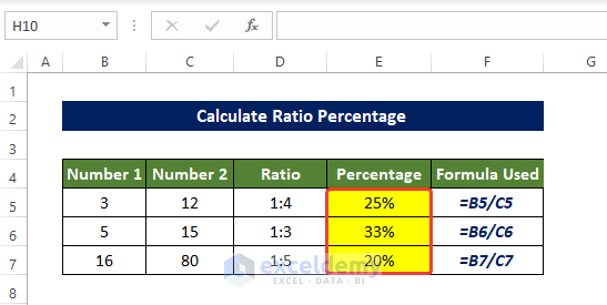
Result
- The range E5:E7 now shows the percentage value of Number 1 relative to Number 2.
Breakdown of the Formula
The GCD(B5,C5) function finds the greatest common divisor, and the formula B5/GCD(B5,C5) and C5/GCD(B5,C5) give us the ratio values.
The final formula B5/GCD(B5,C5)&“:”&C5/GCD(B5,C5) combines these values with the ratio sign “:”.
You can use this method to calculate ratio percentages in Excel.
Read More: How to Convert Percentage to Ratio in Excel
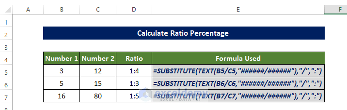
Method 2 – Combining SUBSTITUTE and TEXT Functions
Step-by-Step Calculation
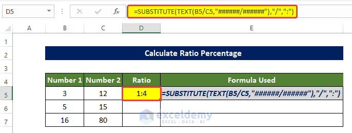
- In cell D5, enter the following formula:
=SUBSTITUTE(TEXT(B5/C5,"######/######"),"/",":")
This formula calculates the ratio between cell B5 and C5 and formats it as a:b (replacing “/” with “:”).
- Drag the Fill Handle down to cell D7 to fill the entire range (D5:D7) with ratios.
- In cell E5, enter the formula:
=B5/C5This calculates the quotient of Number 1 divided by Number 2.
- Drag the Fill Handle down to cell E7 to fill the entire range (E5:E7) with quotient values.
- Select the range E5:E7, go to the Home tab, and click the “%” (Percentage) sign in the Number group.
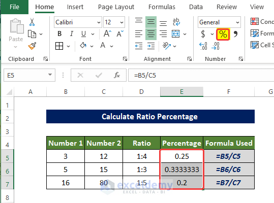
- This converts the quotient values to percentages.
Breakdown of the Formula
- TEXT(B5/C5,”######/######”): This function will return the quotient of the division of the cell B5 by C5 and format it as a fraction.
- SUBSTITUTE(TEXT(B5/C5,”######/######”),”/”,”:”): This formula will substitute the “/” with the “:” in the fraction.
Read More: How to Convert Ratio to Decimal in Excel
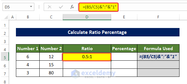
Method 3 – Applying Simple Division
Step-by-Step Calculation
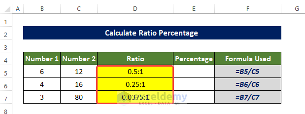
- In cell D5, enter the formula:
=(B5/C5)&":"&"1"This expresses the ratio of Number 1 to Number 2 with respect to 1.
- Drag the Fill Handle down to cell D7 to fill the entire range (D5:D7) with ratios.
- In cell E5, enter the formula:
=B5/C5This calculates the quotient as before.
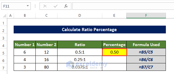
- Drag the Fill Handle down to cell E7 to fill the entire range (E5:E7) with quotient values.
- Select the range D5:D7, and click the percentage icon from the Home tab.
- Now the range E5:E7 shows the percentages of Number 1 relative to Number 2.
Read More: How to Do Ratio Analysis in Excel Sheet Format
Method 4 – Using Combined Formula
Step-by-Step Calculation
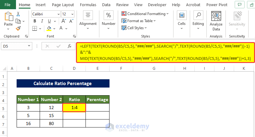
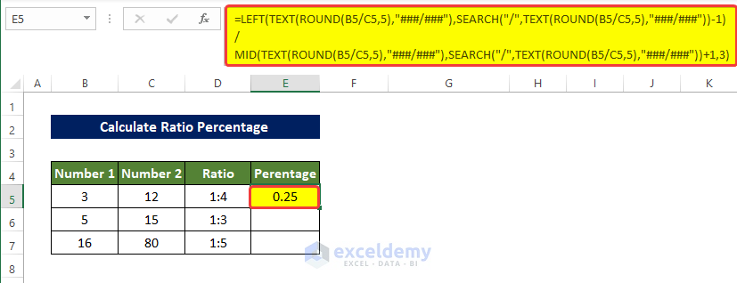
- In cell D5, enter the following formula:
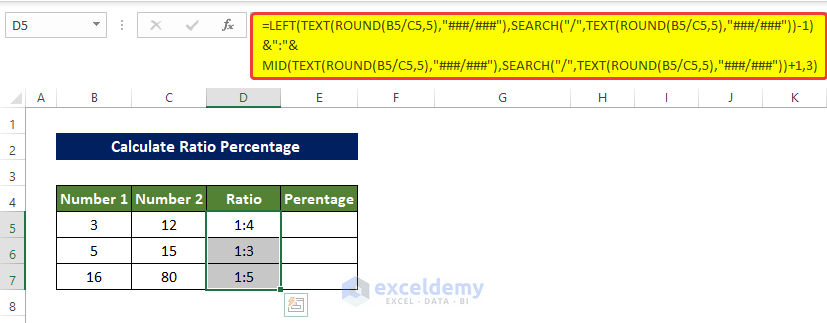
=LEFT(TEXT(ROUND(B5/C5,5),"###/###"),SEARCH("/",TEXT(ROUND(B5/C5,5),"###/###"))-1)&":"&MID(TEXT(ROUND(B5/C5,5),"###/###"),SEARCH("/",TEXT(ROUND(B5/C5,5),"###/###"))+1,3)
This formula calculates the ratio and formats it as a:b.
- Drag the Fill Handle down to cell D7 to fill the entire range (D5:D7) with ratios.
- In cell E5, enter the formula:
=LEFT(TEXT(ROUND(B5/C5,5),"###/###"),SEARCH("/",TEXT(ROUND(B5/C5,5),"###/###"))-1)/MID(TEXT(ROUND(B5/C5,5),"###/###"),SEARCH("/",TEXT(ROUND(B5/C5,5),"###/###"))+1,3)
This calculates the percentages.
- Drag the Fill Handle down to cell E7.
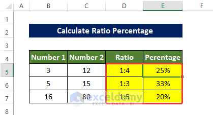
- Select the range E5:E7 and click the percentage icon.
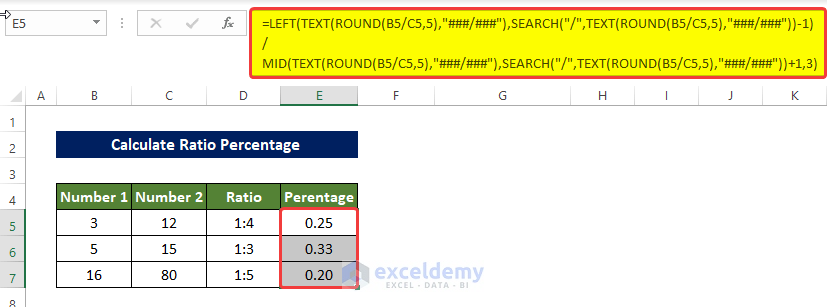
- Now the range E5:E7 shows the percentages of Number 1 relative to Number 2.
Breakdown of the Formula
- ROUND(B5/C5,5):
- This function calculates the quotient of the division of values in cells B5 and C5.
- It rounds the result to 5 decimal places.
- TEXT(ROUND(B5/C5,5),“###/###”):
- The TEXT function formats the rounded quotient as a fraction.
- The format “###/###” ensures that the fraction is displayed correctly.
- SEARCH(“/”,TEXT(ROUND(B5/C5,5),“###/###”)):
- This formula finds the location of the “/” character within the formatted fraction.
- It starts searching from the left side of the text.
- LEFT(TEXT(ROUND(B5/C5,5),“###/###”),SEARCH(“/”,TEXT(ROUND(B5/C5,5),“###/###”))-1):
- The LEFT function extracts the portion of the text from the left side up to the specified location (just before the “/”).
- This gives us the numerator of the ratio.
- MID(TEXT(ROUND(B5/C5,5),“###/###”),SEARCH(“/”,TEXT(ROUND(B5/C5,5),“###/###”))+1,3):
- The MID function extracts a specified section of text from a particular position.
- In this case, it extracts the three characters after the “/” (the denominator of the ratio).
- LEFT(TEXT(ROUND(B5/C5,5),“###/###”),SEARCH(“/”,TEXT(ROUND(B5/C5,5),“###/###”))-1)/MID(TEXT(ROUND(B5/C5,5),“###/###”),SEARCH(“/”,TEXT(ROUND(B5/C5,5),“###/###”))+1,3):
- Finally, this function divides the extracted numerator by the extracted denominator.
- The result is the ratio expressed as “a:b.”
Read More: How to Graph Ratios in Excel
Download Practice Workbook
You can download the practice workbook from here:
Related Articles
<< Go Back to Ratio in Excel | Calculate in Excel | Learn Excel
Get FREE Advanced Excel Exercises with Solutions!

You have an extra 0 in your formula in section 1:
=B5/GCD(B5,C5)&”:”&C5/GCD(B5,C50)
it should read:
=B5/GCD(B5,C5)&”:”&C5/GCD(B5,C5)
Thanks a lot for providing the correction. Both the Image and the Formula has been updated.