How to Calculate Sharpe Ratio in Excel (2 Common Cases)

In this article, we will explain how to calculate the Sharpe Ratio in Excel.

Basics of the Sharpe Ratio

The Sharpe Ratio, also known as the Sharpe Index, is used to calculate the performance of an investment considering all the related risks. It compares investments of different risk profiles against each other.

To calculate the Sharpe Ratio, we use the following formula:

Sharpe Ratio = (Rp - Rf) / Ꝺ

Where,
Rp = Expected Rate of Return
Rf = Risk-Free Rate of Return
Ꝺ = Standard Deviation

A higher value indicates a better investment, representing greater outcomes for the portfolio compared to the inherent risk.

How to Calculate the Sharpe Ratio in Excel: 2 Common Cases

Example 1 – Using a Formula to Calculate the Sharpe Ratio with Known Values

When the values are known, we can simply calculate the Sharpe Ratio by putting the values in the equation.

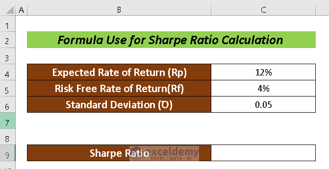
Here, we have a dataset with a given Expected Rate of Return, Risk Free Rate of Return, and Standard Deviation. We can apply the formula above to calculate the Shape Ratio.

Steps:

Select an output cell for the Sharpe Ratio (i.e. C9).
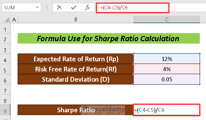
Input the following formula in cell C9:

=(C4-C5)/C6

Where,
C4 = Expected Rate of Return
C5 = Risk-Free Rate of Return
C6 = Standard Deviation

Press ENTER.

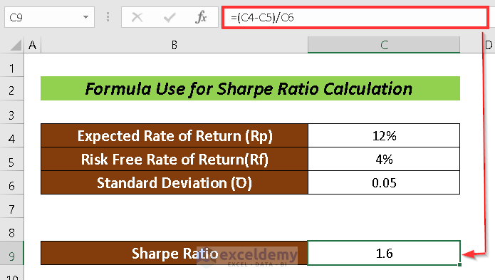
Thus, we can easily calculate the Sharpe Ratio.

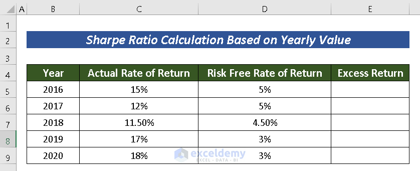
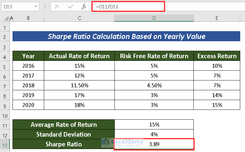
Example 2 – Sharpe Ratio Calculation Based on Yearly Returns

We can also calculate the Sharpe Ratio considering the previous years’ records. Generally, when calculating the Sharpe Ratio based on years, a dataset with an Actual Rate of Return, Risk Free Rate of Return will be provided.

Actual Rate of Return means the change in percentage of the actual investment, and Risk Free Rate of Return means the hypothetical rate of return if there was no risk.

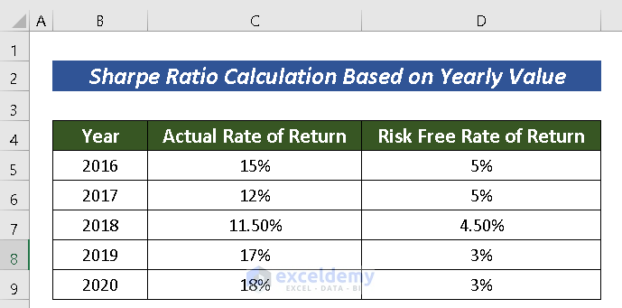
Let’s calculate the Sharpe Ratio for the dataset above.

Steps:

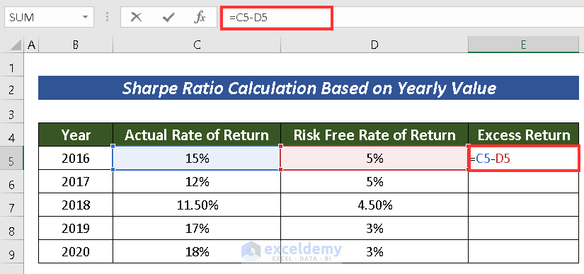
Create an additional column named Excess Return.

In cell E5, enter the following formula to calculate the Excess Return:

=C5-D5

Where,
C5 = Actual Rate of Return
D5 = Risk-Free Rate of Return

Press ENTER.

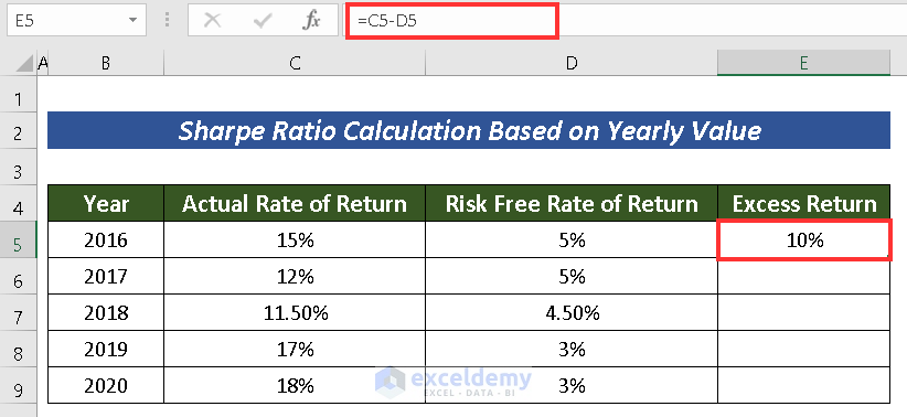
Use the Fill Handle to AutoFill the rest of the cells below.
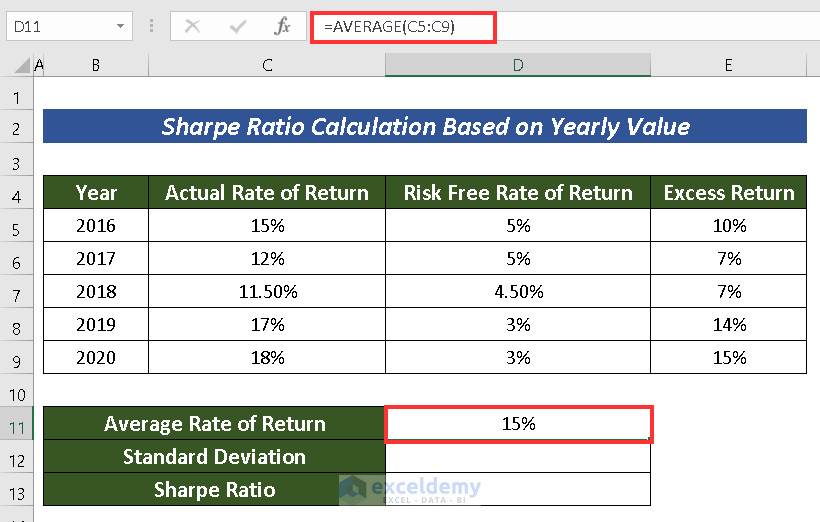
In cell D11, enter the following formula to calculate the Average Rate of Return:

=AVERAGE(C5:C9)

Where the mean value of the cells C5:C9 is calculated.

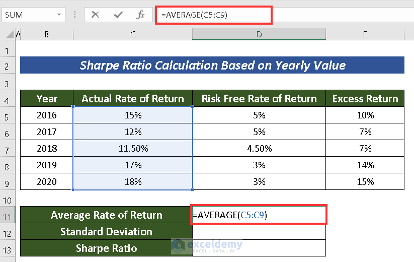
Press ENTER.

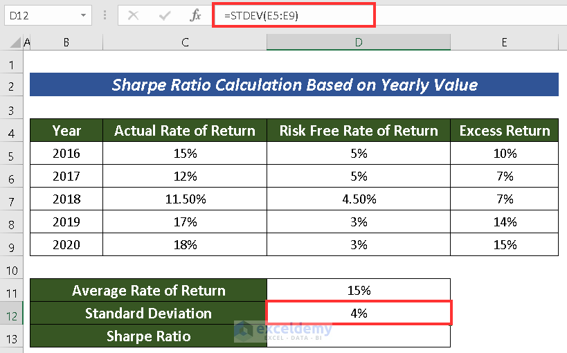
Enter the following formula to calculate the Standard Deviation from the Excess Return:

=STDEV(E5:E9)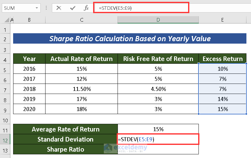

Press ENTER.

Finally, in cell D13, use the following formula to calculate the Sharpe Ratio:

=D11/D12

Where,
D11 = Average Rate of Return

D12 = Standard Deviation

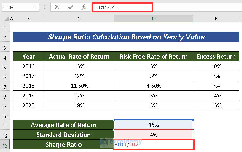
Press ENTER to return our desired output.

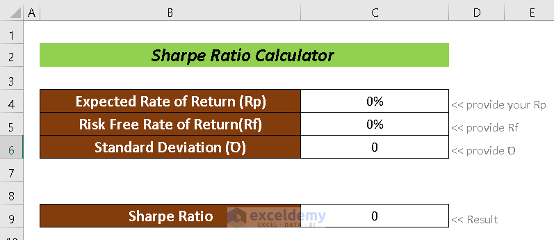
Sharpe Ratio Calculator

We have created a Sharpe Ratio Calculator, which you will find within the provided practice workbook. Simply input the required variables to obtain the Sharpe Ratio.