How to Do Ratio Analysis in Excel Sheet Format (with Quick Steps)

Ratio analysis is a vital task in any organization. It helps us to predict the institution’s strengths and capabilities. In this article, we demonstrate to you how to do ratio analysis in Excel sheet format. If you are interested in estimating your own company’s ratio analysis yourself, download our free template and follow us.

Overview of Ratio Analysis

We deal with several types of reports regarding our organization. Among them, ratio analysis is a significant one. It is mainly a financial statement analysis report of that company that reflects the growth rate, strength, and production capabilities. In this report, we have to estimate four different types of ratios. They are discussed below:

1. Profitability Ratios

The elements of the profitability ratio show us the efficiency of that company in using its assets to make a profit. There are six major items that we will calculate here.

Gross Margin

Gross margin is the ratio of the difference between Sales and Cost of Goods Sold (COGS) with Sales. The mathematical expression of gross margin is:

Operating Profit Margin

Operating Profit Margin is the ratio of the Earning Before Interest & Tax (EBIT) and Sales. The formula to evaluate the ratio is:

Net Margin

This is the ratio of Net Income and Sales. The expression is:

Return on Total Assets

Return on Total Assets or ROA is the ratio of the Earning Before Interest & Tax (EBIT) and Total Assets. The mathematical formula to estimate the ratio is:

Return on Total Equity

Return on Total Equity or ROE is the ratio of Net Income and Net Equity. The formula is shown below:

2. Efficiency Ratios

The ratios show us how efficiently an organization uses its current assets or inventories in cash. We will estimate six elements in this efficiency ratio. They are:

Receivables Turnover Ratio

The receivables Turnover Ratio is the ratio of Sales and Accounts Receivable. Its mathematical formula is:

Inventory Turnover Ratio

It is the ratio of Cost of Goods Sold (COGS) and Inventories. The expression is:

Payable Turnover Ratio

The Payable Turnover Ratio is the ratio of Cost of Goods Sold (COGS) and Accounts Payable. Its mathematical formula is shown below:

Asset Turnover Ratio

The Asset Turnover Ratio is determined by the ratio of Sales and Total Assets. Its calculation expression is:

Fixed Asset Turnover Ratio

The Fixed Asset Turnover Ratio is the ratio of Sales and Net Fixed Assets. The formula to figure out the value is:

Equity Turnover Ratio

The ratio of Sales and Net Equity is called Equity Turnover Ratio. The expression is given below:

3. Liquidity Ratios

Liquidity Ratios define the organization’s cash level, liquidity position, and capability to meet the short-term liabilities. We will calculate three ratios here.

Current Ratio

The Current Ratio is the ratio of Current Assets and Current Liabilities. Its mathematical formula is:

Quick Ratio

The Quick Ratio is the ratio of the combination of Cash and Cash Equivalents & Accounts Receivables with Current Liabilities. The expression is given below:

Cash Ratio

Cash and Cash Equivalents with Current Liabilities is called a Cash Ratio. The formula is:

4. Solvency Ratios

This ratio value tells us whether the organization has the capability to fulfill its long-term responsibilities by comparing the debt level with its total assets & equity. This ratio has three elements.

Debt-To-Equity Ratio

The Debt-To-Equity Ratio is the ratio of  Total Debt and Net Equity. The formula to determine the ratio is:

Debt Ratio

The ratio of Total Debt and Total Assets is known as a Debt Ratio. Its mathematical expression is:

Interest Coverage Ratio

The ratio of Earnings Before Interest, Taxes, Depreciation, And Amortization (EBITDA) and Interest Expenses is called Interest Coverage Ratio. The formula for the interest coverage ratio is:

Advantages of Ratio Analysis

The advantage of making a ratio analysis report is given below:

• Show the strength of the organization.
• Estimate the earning capability.
• The report simplifies the financial statement report.
• Help to compare with a similar type of institution.

Similar Readings

• How to Use Interest Coverage Ratio Formula in Excel
• Debt Service Coverage Ratio Formula in Excel

Step-by-Step Procedure to Do Ratio Analysis in Excel Sheet Format

To demonstrate the process of ratio analysis, we consider an organization’s growth and account data. The whole analysis process is described below step by step. Make sure you use the Absolute Cell Reference sign in the formula to avoid the unpredictable modification of cell reference.

Step 1: Input All Required Particulars

In this step, we will input all the required specifications into Microsoft Excel.

• First of all, launch Microsoft Excel on your device and rename the sheet according to your desire. We entitled our sheet as Specification. The modification of the sheet’s name is not mandatory. It makes your datasheet more convenient for others.
• Then, entitle your dataset with a suitable title. For that, select the range of cells B2:C2 and click on the Merge & Center option from the Alignment group, located in the Home We keep our dataset title as Ratio Analysis Data.

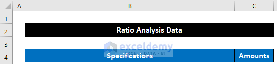
• After that, title cells B4 and C4 as Specifications and Amounts respectively.

• Now, input all the particular values for your organization, denoted in the range of cells B5:B20.

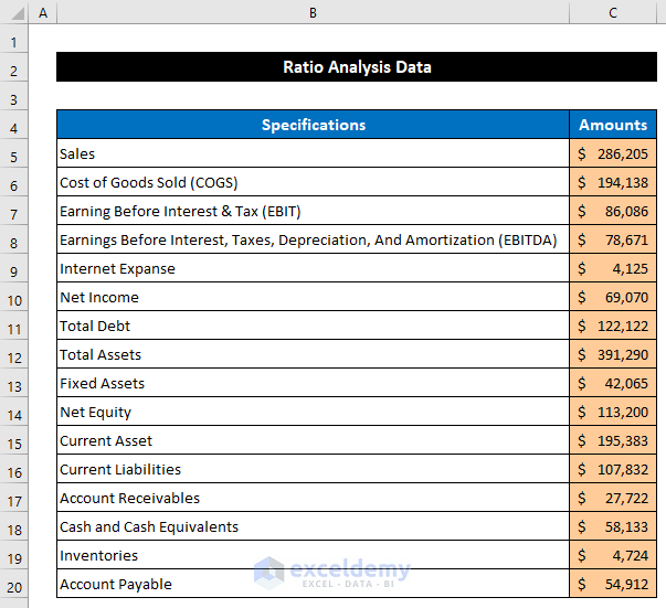
You have completed the first step of ratio analysis in Excel sheet format.

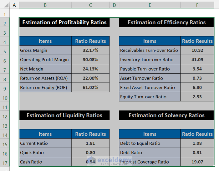
Step 2: Calculate All Profitability Ratios

Here, we will evaluate all the Profitability Ratios. There are five elements in the Profitability Ratio. We will calculate them one by one.

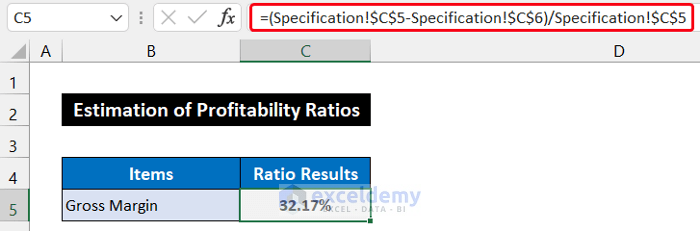
• First, we will calculate the Gross Margin. For that, select cell C5.
• Now, write down the following formula in the cell.

• Press Enter to get the Gross Margin.

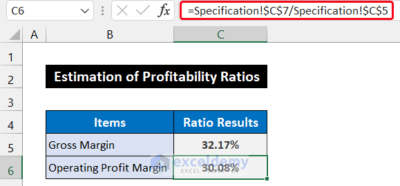
• Secondly, to calculate the Operating Profit Margin, select cell C6 and write down the following formula:

• Press the Enter, and you will get the value.

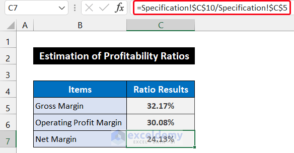
• Next, we are going to determine the Net Margin in cell C7. The formula for calculation is shown below:

• Then, press the Enter to get the result.

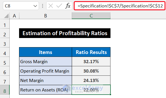
• After that, to estimate the Return on Assets or ROA, write the following formula into cell C8.

• Press Enter on the keyboard.

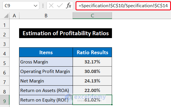
• Finally, for Return on Equity or ROE write down the following formula into cell C9.

• Finally, press Enter to get the value of ROE.

Thus, we can say that you have finished the second step of ratio analysis in Excel sheet format and calculated all the required elements of the Profitability Ratio.

Read More: How to Calculate Ratio Percentage in Excel

Step 3: Evaluate Every Efficiency Ratio

In this following step, we will calculate all the Efficiency Ratios. The Efficiency Ratio contains six elements. We are going to find their value one by one.

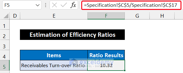
• In the beginning, we will determine the Receivables Turn-over Ratio. To estimate its value, select cell F5.
• Then, write down the following formula in the cell.

• Press Enter to get the value of the Receivables Turn-over Ratio.

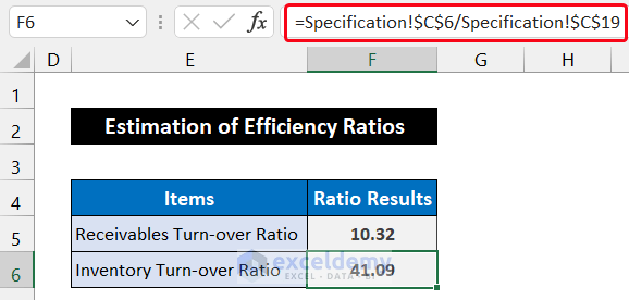
• Next, to figure out the Inventory Turn-over Ratio, select cell F6 and write down the following formula:

• Similarly, press the Enter, and you will get the value.

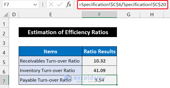
• After that, we are going to determine the Payable Turn-over Ratio in cell F7. The formula for calculation is shown below:

• Press the Enter to get the ratio result.

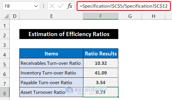
• Our next item is the Asset Turnover Ratio. To estimate its value, write the following formula into cell F8.

• Now, press Enter on the keyboard.

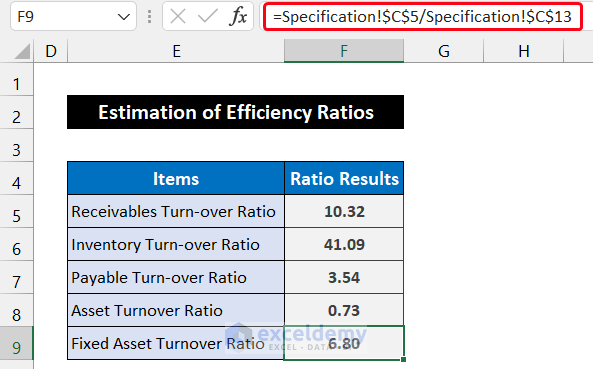
• Next, to evaluate the value of the Fixed Asset Turnover Ratio, write down the following formula in cell F9.

• Again, press Enter to get the value of the Fixed Asset Turnover Ratio.

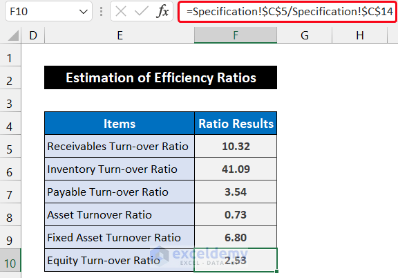
• At last, to compute the Equity Turn-over Ratio, write down the following formula in cell F10.

• Press Enter to get the value of the Equity Turn-over Ratio.

Finally, we can say that you have completed the third step of ratio analysis in Excel sheet format and calculated all six required elements of the Efficiency Ratio.

Read More: How to Convert Ratio to Decimal in Excel

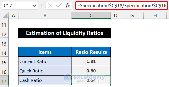
Step 4: Determine Liquidity Ratios

In this step, we are going to figure out all the Liquidity Ratios. In the Liquidity Ratio, we have to find three elements. They are Current, Quick, and Cash Ratios. The calculation is given as follows:

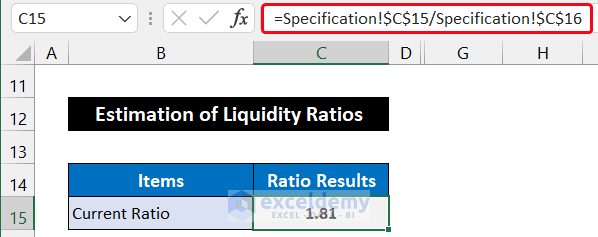
• First, we are going to calculate the Current Ratio. For that, select cell C15.
• Now, write down the following formula into the cell.

• Then, press Enter to get the ratio value.

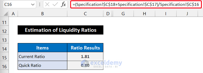
• After that, to figure out the Quick Ratio, select cell C16 and write down the following formula:

• Similarly, press the Enter, and you will get the value of Quick Ratio.

• Next, we will determine the Cash Ratio in cell C17. The formula to calculate the Cash Ratio is shown below:

• Finally, press the Enter to get the ratio result.

At last, we can say that you have accomplished the fourth step of ratio analysis in Excel sheet format and successfully estimated all three required items of the Liquidity Ratio.

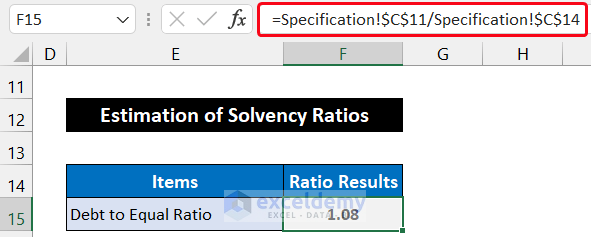
Step 5: Estimate Solvency Ratios

In this final calculation step. We have to evaluate the Solvency Ratios. In the Solvency Ratio, we will find three elements like the previous ratio. Their calculation procedure is given below:

• At first, we will find the Debt to Equal Ratio. For that, select cell F15.
• After that, write down the following formula into the cell.

• Now, press Enter and you will get the ratio’s value.

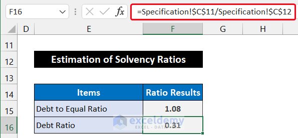
• Then, to get the Debt Ratio, select cell F16 and write down the following formula:

• Similarly, press the Enter, and you will get the value.

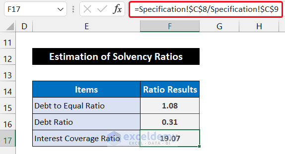
• Finally, we will determine the Interest Coverage Ratio in cell F17. The formula to calculate the ratio is shown below:

• In the end, press the Enter to get the Interest Coverage Ratio.

At last, we can say that you have fulfilled all the steps of ratio calculation.

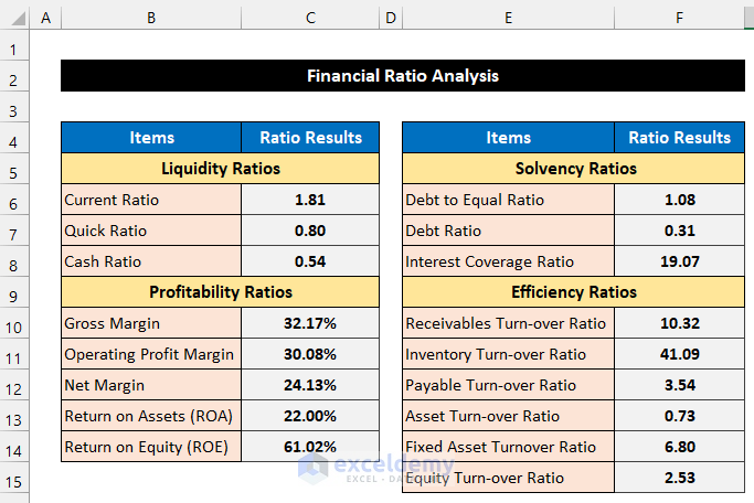
Step 6: Create Ratio Analysis Summary Report

Now, we will create a summary report of our analyzed results with some charts. This summary report is not mandatory. However, we believe that for better visualization of your data and others’ convenience, it is unavoidable. We are going to add three charts to this report. They will be a pie chart, a column chart, and the last one will be a bar chart. The whole process is explained below:

• First, select all four ratio calculation tables in the Ratio Estimation sheet.
• Now, press ‘Ctrl+C’ to copy them.

• Then, create a new sheet. Rename it as Summary, and press ‘Ctrl+V’ to paste them there.
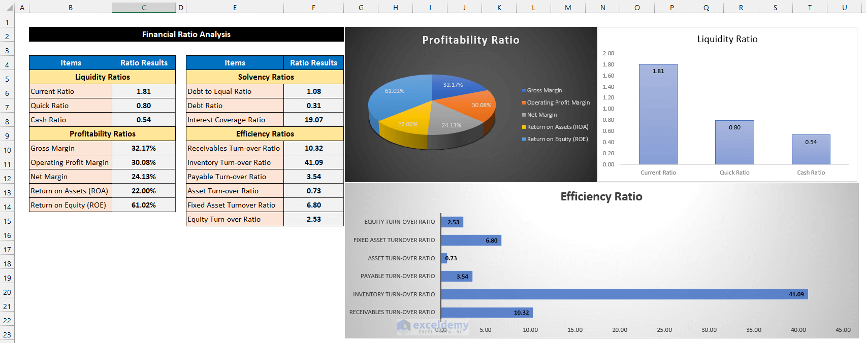
• Format them according to your desire. Our formatting for this report is shown in the image below.

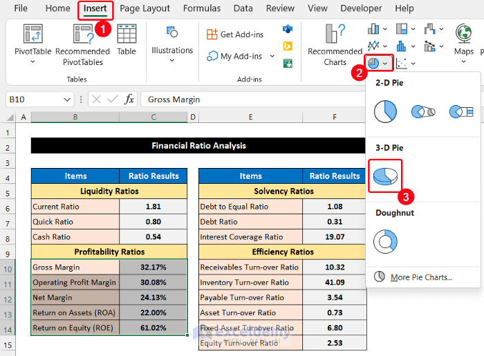
• Now, select the range of cells B10:C14.
• Then, in the Insert tab, select the drop-down arrow of the Insert Pie or Doughnut Chart option and choose the 3-D Pie option.

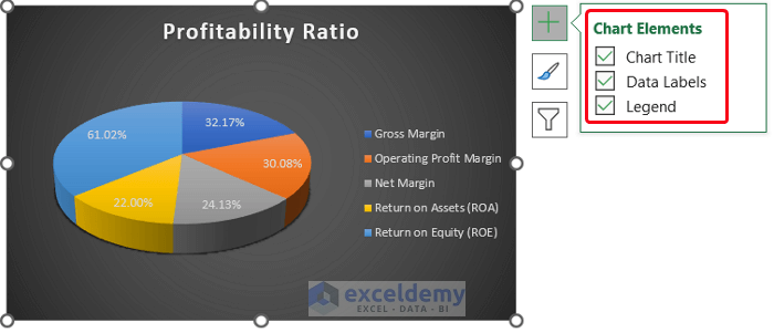
• The chart will appear in front of you. Set a suitable name for your chart. We set our chart title as Profitability Ratio.
• You can also modify your chart style and texts from the Design and Format tabs.
• We chose Style 8 for our chart. For that, select the Style 8 option from the Chart Styles group.

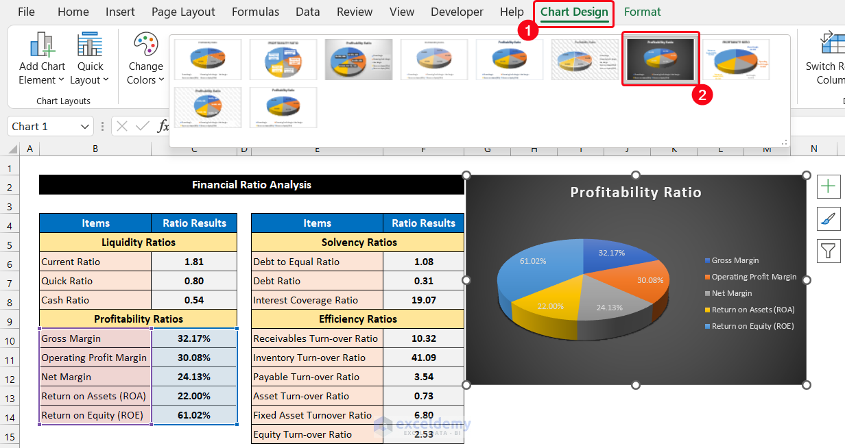
• Besides that, we keep all the Chart Elements for the convenience of other users.

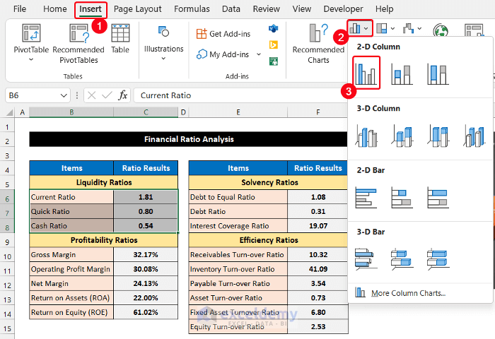
• Next, for the column chart, select the range of cells B6:C8.
• In the Insert tab, select the drop-down arrow of the Column or Bar Chart from the Charts group.
• Then, select the Clustered Column option from the 2-D Column section.

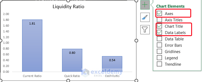
• The chart will come. After that, click on the Chart Element icon and check on the Axes, chart title, and Data Table elements.
• Set the chart title as Liquidity Ratio.

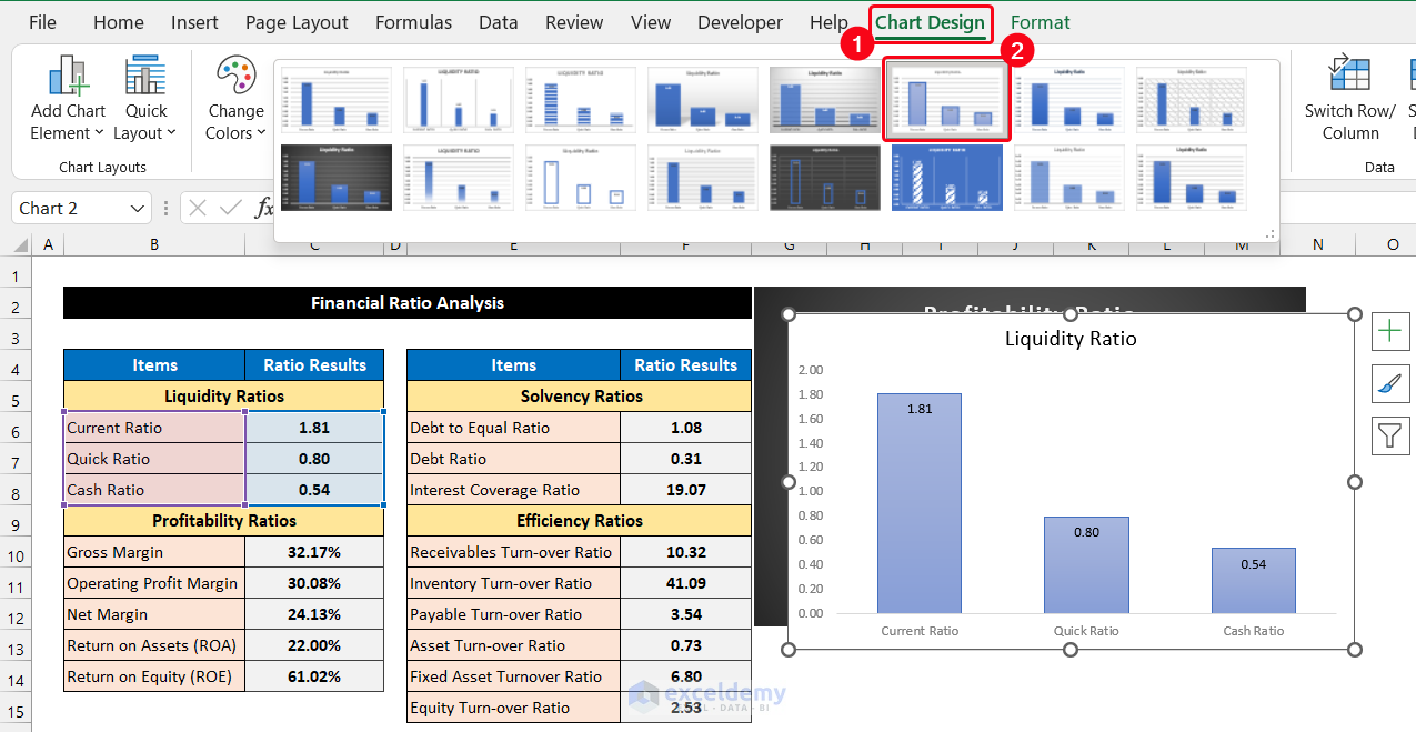
• Besides it, we choose the Style 6 option from the Chart Styles group for our column chart.

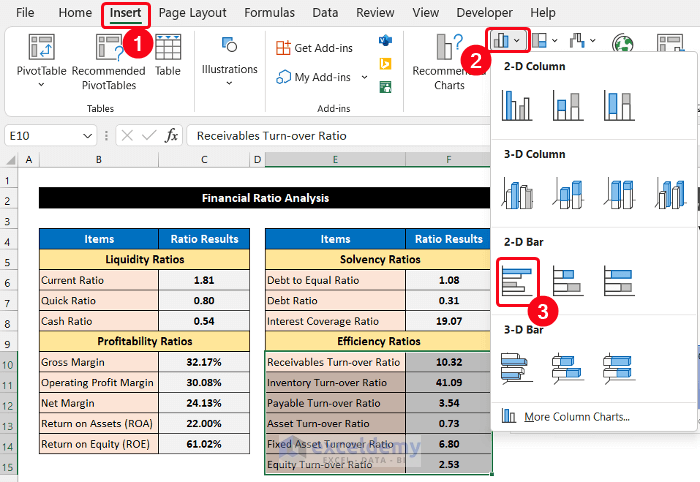
• Finally, for the bar chart, select the range of cells B10:C15.
• In the same process select the drop-down arrow of Columns or Bar Chart, and select the Clustered Bar option from the 2-D Bar section.

• Now, modify the number of elements and the chart style according to your desire. We choose Style 3 and the Axes, chart title, and Data Table elements in this chart.

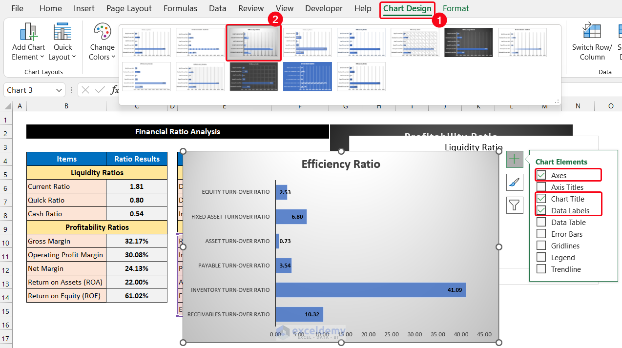
• Finally, use the Resize icon at the edge of the chart for better visualization and complete the task.

Finally, we can say that we have completed all the steps properly and we can perform ratio analysis in Excel sheet format.

Download Practice Workbook

Conclusion

That’s the end of this article. I hope that this article will be helpful for you and you will be able to do ratio analysis in Excel sheet format. Please share any further queries or recommendations with us in the comments section below if you have any further questions or recommendations. Keep learning new methods and keep growing!

Related Articles

• How to Graph Ratios in Excel
• How to Use Interest Coverage Ratio Formula in Excel
• Debt Service Coverage Ratio Formula in Excel
• How to Convert Percentage to Ratio in Excel

<< Go Back to Ratio in Excel | Calculate in Excel | Learn Excel