This tutorial will demonstrate how to calculate break-even analysis using formula in Excel. Break-even is one of the most important parameters for running a business company. When you start a business, the first target becomes that you try to run your business without any loss. For that, you need to know the break-even point in excel for your business. This is the best parameter to determine whether the business is running profitably or with a loss. So, it is extremely essential to perform a break-even analysis Excel formula in Excel.
What Is Break Even Analysis?
While running a business, you have to measure whether your company is at a loss or not. To determine that, the most useful method is the break-even analysis. Break-even analysis means your earnings are equal to the money you have spent in the business. In simple words, if the profit is exactly zero then it is called the break-even point. If you have a profit higher than the break-even point, then you are running your business profitably but if you have a profit lower than the break-even point, then you are running your business at a loss. So, with the break-even analysis, you can easily understand the situation of your company and make decisions accordingly.
How to Perform Break-Even Analysis with Formula in Excel: 3 Effective Methods
We’ll use a sample dataset overview as an example in Excel to understand easily. If you follow the steps correctly, you should learn how to perform the break-even analysis Excel formula in Excel on your own. The methods are described thoroughly below.
1. Using Goal-Seek Feature to Perform Break-Even Analysis
In this case, our goal is to perform the break-even analysis by using the Goal-Seek feature in Excel. This feature is very useful in times when we want to find a specific input for the available output. We can learn this method by following the below steps.
Steps:
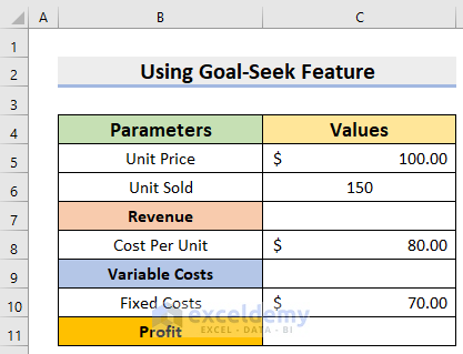
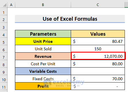
- First, we arranged a dataset like the below image. In this case, we have the Parameters in column B and Values in column C. Moreover, in cells B5, B6, B7, B8, B9, B10, and B11 we have sequentially Unit Prices, Unit Sold, Revenue, Cost Per unit, Variable Costs, Fixed Costs, and Profit.
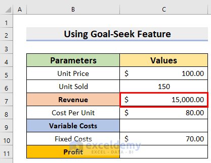
- Next, insert the following formula in the C7 cell.
=C5*C6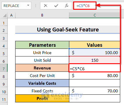
- After that, you will get the result for this cell by using the multiplication of two cells.
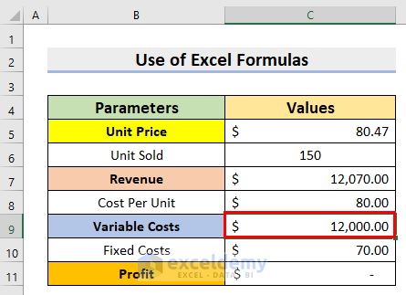
- Then, insert the following formula in the C9 cell.
=C6*C8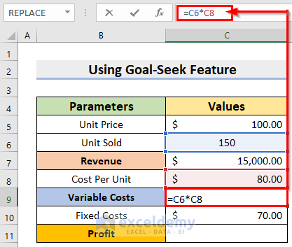
- Afterward, you will get the result for this cell with the help of the multiplication of two cells.
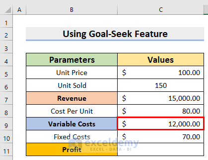
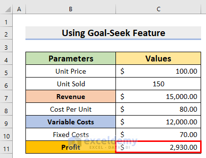
- Subsequently, insert the following formula in the C11 cell.
=C7-C9-C10
- Furthermore, you will get the result for this cell by using substructions of C9 and C10 cells from the C7 cell.
- Moreover, go to Data >> What-if Analysis >> Goal Seek options.
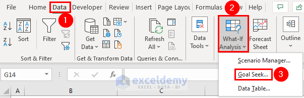
- Therefore, in the Goal Seek dialog box, set the cell you want to change( in this case cell C11 named Profit) in the Set Cell Moreover, in the To value option, select the data you want to achieve. In the By changing cell option, insert the cell number you want to use as a source of the change(in this case cell C5 named Unit Price).

- Hence, if you press the Enter button, in the Goal Seek Status dialog box, you will get the result and click on the OK option there.

- Finally, you will get the result for this cell with the help of the Goal Seek feature in Excel. It shows us the minimum Unit Price and minimum Revenue at which the profit is zero. If we want to do a profit in our business, we have to mark the Unit Price and Revenue higher than the results.
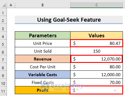
Thus, we have performed the break-even analysis Excel by using the Goal-Seek feature in Excel.
Read More: How to Do Multi-Product Break Even Analysis in Excel
2. Determining Break-Even Analysis by Excel Formula
Now, we want to determine break-even analysis in Excel by using formulas. We can fulfill our goal by following the below steps.
Steps:
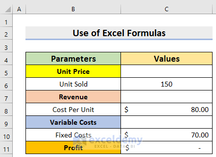
- At first, we arranged a dataset like the below image. In this case, we have the Parameters in column B and Values in column C. Moreover, in cells B5, B6, B7, B8, B9, B10, and B11 we have sequentially Unit Prices, Unit Sold, Revenue, Cost Per unit, Variable Costs, Fixed Costs, and Profit.
- Then, insert the following formula in the C5 cell.
=C10/C6+C8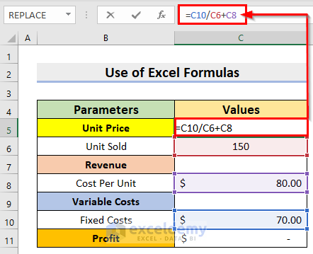
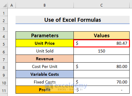
- Now, you will get the result for this cell with the help of the division of cells.
- After that, insert the following formula in the C7 cell.
=C5*C6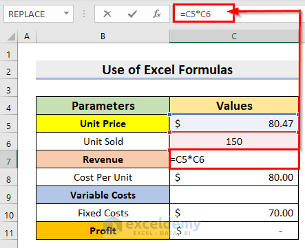
- Next, you will get the result for this cell with the help of the multiplication of two cells.
- Therefore, insert the following formula in the C9 cell.
=C6*C8
- Last, you will get the result for this cell with the help of the multiplication of two cells. It shows us the minimum Unit Price and minimum Revenue at which the profit is zero. With this, we have found out the minimum Variable Costs in the business. If we want to do a profit in our business, we have to mark the Unit Price, Revenue, and Variable costs higher than the results.
Therefore, we have determined the break-even analysis in Excel by using formulas.
Read More: How to Do NPV Break-Even Analysis in Excel
3. Break Even Analysis with Excel Chart
Next, we want to determine break-even analysis in Excel by using charts. We can fulfill our goal by following the below steps.
Steps:
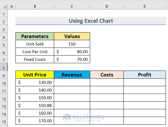
- To begin with, we arranged a dataset like the below image. In this case, we have the Parameters in column B and Values in column C. Moreover, in cells B9, C9, D9, and E9 we have sequentially Unit Prices, Revenue, Costs, and Profit.
- In addition, insert the following formula in the C10 cell.
=B10*$C$6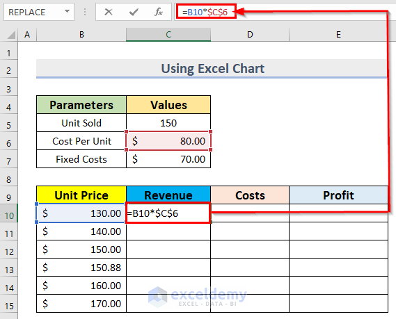
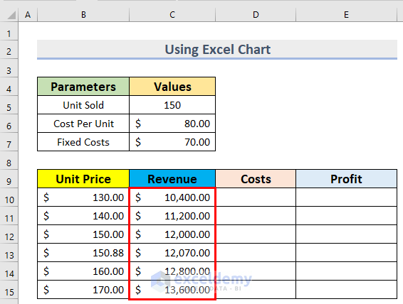
- Furthermore, you will get the result for this cell with the help of the multiplication of two cells and then use the Fill Handle to apply the formula to all the cells.
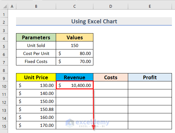
- Subsequently, you will get the proper Revenue for all cells of this column.
- Hence, insert the following formula in the D10 cell.
=$C$5*$C$6+$C$7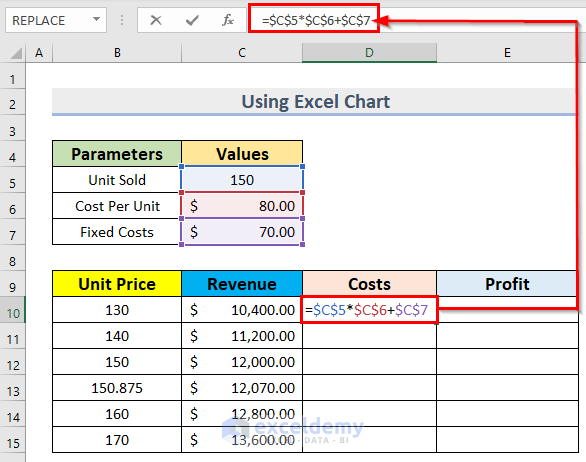
- Now, you will get the result for this cell with the help of the addition of cells, and then use the Fill Handle to apply the formula to all the cells.

- After that, you will get the proper Costs for all cells of this column.

- Thereafter, insert the following formula in the E10 cell.
=C10-D10
- As a result, you will get the result for this cell with the help of the subtraction of two cells and then use the Fill Handle to apply the formula to all the cells.

- Therefore, you will get the proper Profit for all cells of this column.

- Presently, select the data table and then go to Insert tab.

- Consequently, select the Scatter chart from the Insert tab.

- Now, you will get the chart accordingly.

- Additionally, select the intersection point in the chart. Then, right-click on the point and select Add Data Callout from the Add Data Label option in Excel.

- Finally, you will get the insertion point marked here in the chart. The result 875 represents the break-even unit cost and 12,070 represents the break-even Revenue cost in the chart. If we want to run the business profitably, then we have to keep the Unit costs and Revenue more than the results we have found.

As a result, we have determined the break-even analysis in Excel by using charts.
How to Calculate Payback Period in Excel
At this point in the article, our goal is to calculate the payback period in Excel. We can do this by using different formulas in different sections. We want to use COUNTIF, VLOOKUP, and ABS functions in Excel. The COUNTIF function counts the number of cells under certain conditions in Excel. The VLOOKUP function is mainly used to find a certain value from a range of data. We will use the ABS function to get the absolute results. We will describe the whole process by following the below steps.
Steps:
- At first, we arranged a dataset similar to the below image. In this case, we have Year, Cash Inflows, Cash Outflows, and Net Cash Flow sequentially in columns B, C, D, and E.

- Then, insert the following formula in the D12 cell.
=COUNTIF(E5:E10,"<0")
- Moreover, you will get the result for this cell using the COUNTIF function.

- Furthermore, insert the following formula in the D13 cell.
=VLOOKUP(D12, B5:E10, 4)
- As a result, you will get the result for this cell using the VLOOKUP function.

- Therefore, insert the following formula in the D14 cell.
=VLOOKUP(D12+1, B5:E10, 2)
- So, again, you will get the result for this cell using the VLOOKUP function.

- Hence, insert the following formula in the D15 cell.
=ABS(D13/D14)
- Next to that, you will get the result for this cell using the ABS function.

- Additionally, insert the following formula in the D16 cell.
=D12 + D15
- Afterward, you will get the result for this cell using the addition of two cells.

- Therefore, insert the following formula in the D17 cell.
=D16*12
- Last, you will get the result for this cell using the multiplication of cells.

Therefore, we have calculated the payback period in Excel by the use of the COUNTIF, VLOOKUP, and ABS functions in Excel.
Download Practice Workbook
You can download the practice workbook from here.
Conclusion
Henceforth, we have described all methods that will help you to show a break-even analysis Excel formula. We will be glad to know if you can execute the task in any other way. Please feel free to add comments, suggestions, or questions in the section below if you have any confusion or face any problems. We will try our best to solve the problem or work with your suggestions.
Related Articles
<< Go Back To Break Even Analysis Excel | Excel For Finance | Learn Excel
Get FREE Advanced Excel Exercises with Solutions!
