How to Do a Multi-Product Break-Even Analysis in Excel (Step-by-Step Guide)

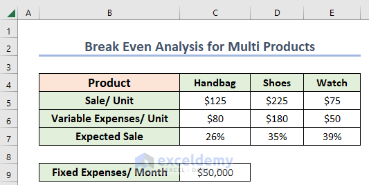
The following dataset contains information on per-unit sales, per-unit variable expenses, and the expected sale ratio of 3 products, along with the company’s fixed expenses per month.

Step 1: Compute the Weighted Average Selling Price

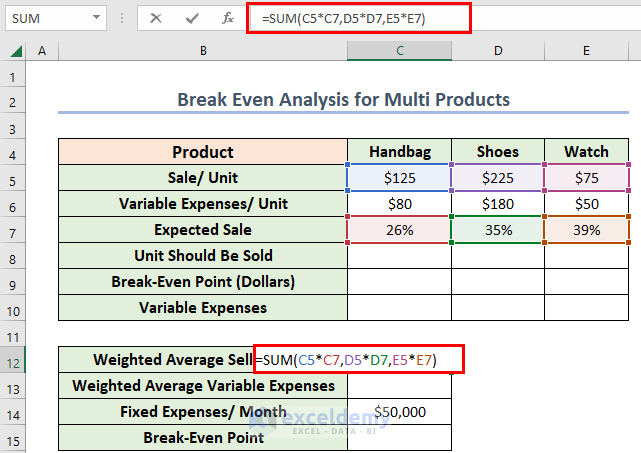
• Select cell C12, where you want to keep the weighted average selling price.
• Enter the formula given below in cell C12.

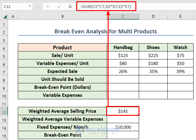
In this formula, I have multiplied the unit sale by the expected sale for each product. Then, I used the SUM Function to add them.

• Press ENTER, and you will see the weighted average selling price.

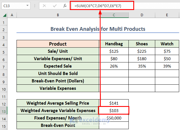
Step 2: Obtain the Weighted Average Variable Expenses

• Select cell C13, where you want to keep the weighted average variable expenses.
• Enter the formula given below in cell C13.

In this formula, I multiplied the unit variable expense by the expected sale for each product and used the SUM function to add them.

• Press ENTER to get the result.

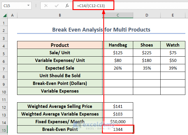
Step 3: Calculate the Break-Even Point

• Select cell C15, where you want to keep the break-even point.
• Enter the following formula in cell C15:

In this formula, I have divided the fixed expenses (per month) by the difference between the weighted average selling price and the weighted average variable expenses.

• Press ENTER, and you will find the break-even point.

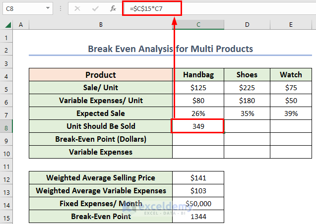
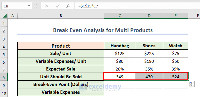
Step 4: Determine the Product Amount That Should Be Sold

• Select cell C8, where you want to keep the target unit.
• Enter the following formula in cell C8:

I have multiplied the break-even point by the expected sale ratio in this formula.

• Press ENTER, and you will find the total unit of handbags that should be sold to balance the cost.

• Drag the Fill Handle icon horizontally to AutoFill the corresponding data in cells D8 and E8.

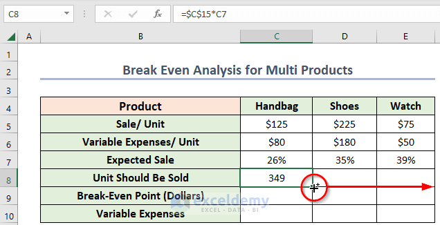
You will get the unit for all the products that should be sold to cover the costs.

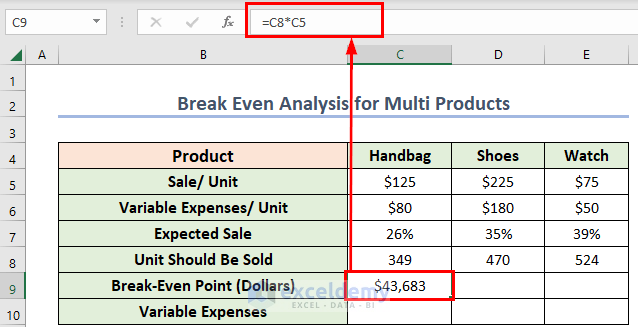
Step 5: Obtain the Total Sales at the Break-Even Point

• Select cell C9 and enter the corresponding formula:

In this formula, I have multiplied the sales per unit by the total target units.

• Press ENTER, and you will find the total sales of handbags.

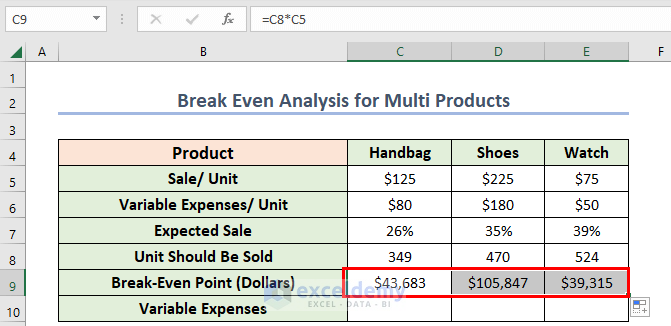
• Drag the Fill Handle icon horizontally to AutoFill the corresponding data in the rest of the cells D9 & E9.

You will get certain sales for all the products to cover the costs.

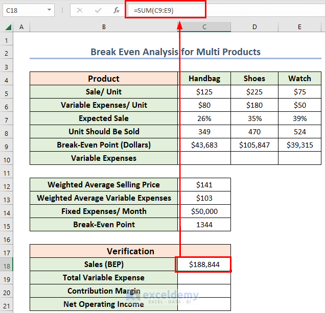
• For sales at the break-even point, use the following formula in cell C18:

In this formula, I have added all the target sales.

• Press ENTER to get the sales (BEP).

Step 6: Calculate the Total Variable Expense

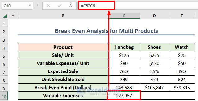
• Select cell C10, where you want to keep the variable expenses for the handbag.
• Enter the formula given below in cell C10:

Here, in this formula, I have multiplied variable expenses per unit by total target units.

• Press ENTER to get the result.

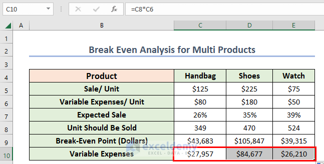
• Drag the Fill Handle icon horizontally to AutoFill the corresponding data in cells D10 and E10.

You will get certain variable expenses for all the products.

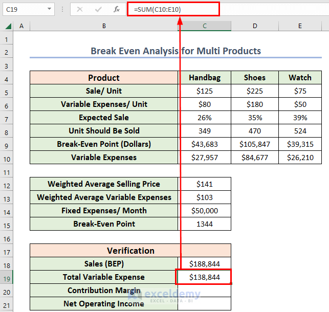
• For total variable expense, enter the following formula in cell C19:

In this formula, I have added each product’s variable expenses.

• Press ENTER to get the total variable expense.

Read More: How to Make a Break-Even Chart in Excel

Step 7: Compute the Contribution Margin

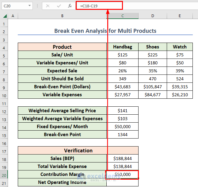
• Select cell C20, where you want to keep the contribution margin.
• Enter the following formula:

In this formula, I have subtracted the total variable expense from the sales at the break-even point.

• Press ENTER, and you will find the contribution margin.

Step 8: Evaluate the Net Income for Verification

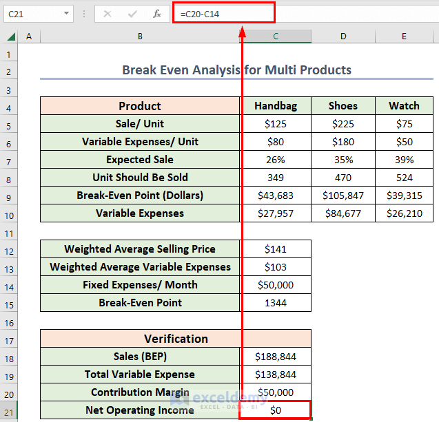
• Select cell C21, where you want to keep the net operating income.
• Enter the following formula in cell C21:

In this formula, I have subtracted the fixed expense from the contribution margin.

• Press ENTER, and you will find the net operating income.

As you can see, the net operating income is zero, so you can say that the break-even analysis is correct.

Read More: How to Do Break Even Analysis with Goal Seek in Excel

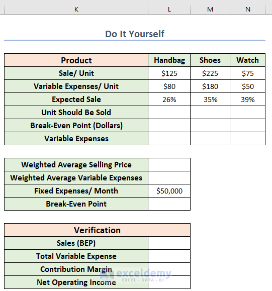
Practice Section

Download the Practice Workbook

You can download the practice workbook from here:

<< Go Back To Break Even Analysis Excel | Excel For Finance | Learn Excel