Latest Posts From Shahriar Abrar Rafid

We will use a sales report for a particular grocery store. This dataset contains the Sales Rep, Order Date, Product Name, and their corresponding Sales amount ...
The name of the sheet is Importing Data to Excel. The dataset includes Sales Rep, Product Name, Unit, and Sales. Step 1 - Change the Privacy of Google ...

Let's use a daily Sales Report of a fast-food shop to demonstrate vertical-to-horizontal copying. Columns B, C, and D of this dataset contain the ...

We will use 2 different CSV files and put them in the same folder. One is File 1, and the other one is File 2. Now, we’ll use these two CSV files to ...

CSV, short for Comma Separated Values, is a widely used file format used to store delimited records in plain text. It is often used to transfer data between ...

Frequently, we need to convert text to columns in Excel in our day-to-day tasks. In fact, Microsoft Excel is an excellent tool to perform this task. Obviously, ...
Clear formatting in Excel means removing the existing formatting and keeping the default formatting. In this Excel tutorial, you will learn how to clear ...
The dataset showcases a Follow-up History of 10 Cancer Patients. 1 and 0 indicate the status of the patient at the time of the last follow-up. ...

Suppose the car tires of a certain company lasted for a mean of 40,000 km and had a standard deviation of 2,500 km. If you buy one tire from this company, what ...

Obviously, you heard the term weather forecasting where weather forecasters determine the likelihood that it will rain, snow, have clouds, etc. on a specific ...

Step 1 - Create the Basic Outline Steps: Give a suitable heading in the B2:G2 range. We’ve put Interim Payment Certificate. In the B4:G7 ...

In this article, we will present 4 easy steps to create a money market interest calculator in Excel. We also provide a free template at the bottom. What ...

Step 1 - Calculate Monthly Income For illustration, we have a sample Monthly Income dataset with a column for sources of income in the B5:B8 range. The income ...

This dataset includes SalesRep’s name, and sales for June and July in columns B, C, and D. Trend arrows can show the increase or decrease in sales. ...
Generic Formula to Calculate the Average True Range The stock's daily high, daily low, and daily close price are needed to calculate the average true range. ...
- « Previous Page
- 1
- 2
- 3
- 4
- 5
- …
- 8
- Next Page »
See Our Reviews at


List of Orders
5/31/22 Trucker A to Destination B Price $250
6/01/22 Trucker A to Destination B Price $300
6/05/22 Trucker A to Destination B Price $400
First, sort your Order Date column by Newest to Oldest order. Then, use Trucker A to Destination B as the lookup value. Now, you’ll get the latest price by using the VLOOKUP function.
Hello AHMED
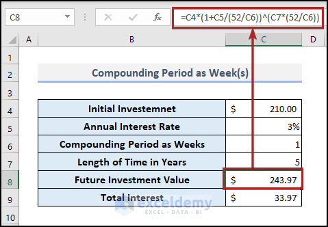
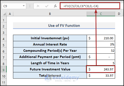
I think you made an unintentional mistake during the calculation.
After 5 years, the future value would be $243.97. The result would come the same whether you calculate manually or use any function.
Calculating manually, you’ll get the result below.
And, using the FV function the result would come like in the one below.
Hello LINCHEN NUMBY,
Thanks for your comment. Here, we’re very eager to help this kind of new startup.
For ease of understanding, you may download the workbook to go along with the approach.
From your comment above, we’ve made an imaginary dataset for your company. Let’s have a look at this first.
Then, construct a new column named Group under Column E.
After that, select cell E5 and enter the following formula.
=IF(D5>5000,"Key Product",IF(D5>=2000,"Large",IF(D5<2000,"Small")))Following this, press ENTER.
Now, bring the cursor to the right-bottom corner of cell E5; instantly, it’ll look like a plus (+) sign. Basically, it’s the Fill Handle tool.
Currently, double-click on it to get results in the following cells also.
Finally, the results are here.
Alternatively, you can use the following formula instead of the previous one.
=IFS(D5>5000,"Key Product",D5>2000,"Large",D5<2000,"Small")So, that’s all from me on this problem. Feel free to contact us for other inquiries. Follow our website Exceldemy to explore more about Excel.
Hello Elaine,
First, it feels good to see your interest in learning it. That motivates us to work hard.
Now, coming back to your question. Here you intend to enter the End Date Status automatically. Yes, that’s a very good thought. In this era of automation, why should we lag behind? Hahahaha…. Okay, let’s get to the solution now.
There could be 4 separate conditions. First, the Last Follow-up Date could be before the End Date of the study and the patient is dead at the Last Follow-up Date. Second, the Last Follow-up Date could be after the End Date of the study and the patient is dead at the Last Follow-up Date. Third, the Last Follow-up Date could be before the End Date of the study and the patient is alive at the Last Follow-up Date. And the fourth, the Last Follow-up Date could be after the End Date of the study and the patient is alive at the Last Follow-up Date. So, how can we determine the End Date Status for these situations? Let’s see the steps below.
• Firstly, go to cell G5 and enter the following formula.
=IFS(AND(E5=1,D5<F5),1,AND(E5=1,D5>F5),0,AND(E5=0,D5<F5),"?",AND(E5=0,D5>F5),0)Here, we used the IFS function where we inserted those 4 conditions as logical_test and their output as value_if_true. Further, we used the AND function to join two conditions together.
• Finally, press ENTER.
That’s all from me on this. Don’t forget to visit our website, Exceldemy, a one-stop Excel solution provider, to explore more.
Stay well and healthy. Happy Excelling ☕.
Hello Jane,
Hope this article is useful for you. I’ve got your problem. The main reason behind it is using the COUNT function. The COUNT function cannot count the Text values. So, you’ve to use the COUNTA function in this case. You may download the workbook for a better understanding. See the following image.
Here, in cell B10, we can see the total count as 0 and in cell C10, the total count is 5. Because in the left cell, we used the COUNT function which is unsuccessful to retrieve the total number of sales reps. But, the COUNTA function in the right cell gives us the right result.
The formula we used in cell B10 is the following.
="Total: "&COUNT(B5:B9)And the formula in cell C10 is given below.
="Total: "&COUNTA(C5:C9)That’s all from me on this topic. Happy Excelling…
Hello Emily,
It is very motivating for us when someone benefits from using our method. Now getting back to your query. You can use a simple copy-paste feature to overcome this issue. Let’s see the process below for a better understanding.
• Firstly, select cells in the C5:C13 range.
• Then, press the CTRL key followed by the C key on the keyboard.
This command copies the whole range.
• After that, right-click on cell E5.
• In the context menu, select Values (V) in the Paste Options.
You can see the data pasted in the new place.
• Additionally, select cells in the B5:B13 range and C4:C13 range also.
• Therefore, delete them using the Delete button.
• At this time, press CTRL+C to copy the cells in the D5:D13 range.
• Henceforth, go to cell B5 and paste them by pressing CTRL+V.
Finally, you get the desired result.
Hello JEFF,
Thank you so much for your valuable contribution to the discussion on our blog. We appreciate you taking the time to share the first code snippet for checking the existence of a worksheet. It’s always great to see different approaches and perspectives being shared, and your code provides an alternative solution to the problem.
If you have a small number of sheets or prefer a more explicit and controlled check, then our code with the loop can still be a valid option. And your approach avoids unnecessary iteration through all sheets and provides a straightforward way to check the existence of a worksheet.
Once again, thank you for your participation and we value the engagement of our readers, and your comment adds even more depth to the topic.
Hope to see more of your valuable contributions in the future!
Regards,
SHAHRIAR ABRAR RAFID
Team ExcelDemy
Hello NOOB Excel,
Thanks for your feedback and sorry for the inconvenience. Now, check the article. We’ve updated it according to your input. Look over it and let us know if it works well for you now.
Regards,
SHAHRIAR ABRAR RAFID
Team ExcelDemy
Hi BARYY,
Thanks for your appreciation. I feel very happy that my tutorial helped you. Now, get back to your query.
Yes, you can simply Copy the worksheet. Assume, we named the worksheet “Jan” for the month of January.
Right-click on the sheet name tab and select Move or Copy from the context menu.
In the Move or Copy dialog box, select move to end and check the box of the Create a copy option. Then, click OK.
But, this procedure is lengthy and time-consuming. Because you have to repeat this process 11 times for the remaining 11 months. Also, you have to rename the sheets according to the month’s name. Instead, you can use a simple VBA macro to do it in a click.
In the Visual Basic Editor, click Insert >> Module.
Paste the following code into the module and click on the Run button.
See the result with your own eyes.
Again, thanks for your query. Your interest in learning is what motivates us to create better content.
Regards,
SHAHRIAR ABRAR RAFID
Team ExcelDemy
Hello GREG,
Thanks for your comment. Yes, you can do it. Here, I’m showing you to do it with Bing Maps API. Because it’s free. To use Google Maps API, you need to register with Card information. So, I have chosen Bing over Google here.
The following VBA macro is the one-stop solution to your problem.
Run this macro and it will ask to input the range containing the latitude and longitude. Make sure to keep a blank column adjacent to the input columns. You’ll get the output there.
Regards,
SHAHRIAR ABRAR RAFID
Team ExcelDemy
Hello NIGEL,
We like to solve this kind of problem and it makes us so happy if it solves your problem.
You can use the following VBA code.
After running the macro, it will pop up a message box asking you to enter the whole range of data. Then you will be asked to enter the number maintaining the sequence. And make sure to enter the numbers without any spaces or commas.
As a result, you will get the calculated frequency in a message box and the row containing the combination will get highlighted.
But, the above code only works for consecutive matches. For example, if you search for 3,4,5 and the values in a row are 3,7,6,4,1,5 then it cannot count this. So, I’ve modified the code to make it usable with all kind of conditions. The following code can calculate the frequency of combination under any criteria.
This code is the ultimate solution for your problem.
Is this the solution you wanted? If you need something else, put the query in the reply.
Regards,
SHAHRIAR ABRAR RAFID
Team ExcelDemy
Hello JEREMY,
Thank you for your comment. I’ve understood your problem. You can use the following instruction. Don’t paste this code into the module. Use it in the sheet module.
Right-click on the sheet name and select the View Code option from the context menu.
Besides, you can double-click on the specific sheet to add a module for this sheet especially.
In the module, paste the following code.
You don’t have to run this code. Simply, save it and return to the worksheet and it’ll work smoothly.
If you delete the data in Column C, the date and time for this particular data will be erased also. But, don’t delete the entire column, it’ll create an error and you have to press CTRL + X to stop the macro from running.
Again, thanks for your query. We always welcome our readers to ask this type of info-ful questions.
Regards,
SHAHRIAR ABRAR RAFID
Team ExcelDemy
Hi SUNITA,
Thank you for your comment and feedback! I appreciate your suggestion regarding including the profit and loss statement alongside the explanation of the balance sheet ratio analysis. It’s a valuable point, and I completely understand how having those additional financial statements would provide a more comprehensive understanding of the topic.
You can go through our article, How to Make Profit and Loss Account and Balance Sheet in Excel to add the profit and loss statement.
Thank you once again for your input!
Regards,
SHAHRIAR ABRAR RAFID
Team ExcelDemy
Hello G,
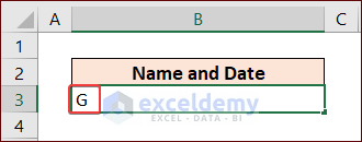
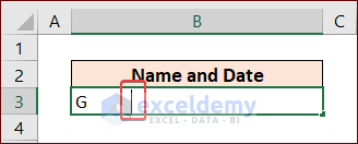
I think that you want to write a name, then some spaces, and then a date in one cell in Excel. Am I right? If that’s the matter, the solution is quite easy.
At first, select the cell (e.g. cell B3) and write your desired name. In this case, we wrote G.
Then, press the SPACE button multiple times according to the space you need. Here, we gave 10 spaces to create an indentation.
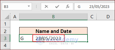
Next, write the date like the following image.
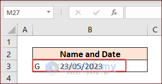
Finally, press the ENTER key. And the ultimate outcome is as follows.
Look, this is quite easy. But, if you want to mean something else, please write specifically. It’ll be helpful for us.
Thanks for your comment.
Regards,
SHAHRIAR ABRAR RAFID
Team ExcelDemy
Hello ROBERT,
Do you have Google API? I think the code works. But if it doesn’t work for you, you can use the simple Import feature which I mentioned in the previous reply.
Even if you want to do it with VBA, you can do it through Google Forms. This process doesn’t require the API key.
If you have further queries, you can comment below. Thanks for your feedback.
Regards
SHAHRIAR ABRAR RAFID
Team ExcelDemy
Hello TANJA,
Hope you are doing good. Thanks for your query.
specifically, which method’s formula isn’t working for you? If you said that, I could understand well. Because all formulas are working on my PC.
The error message “There is a problem with this formula” usually appears when there is an issue with the syntax of the formula. If we take Method 2 as example, the following is the formula we used in cell E5:
=MIN((DATEDIF(C5,TODAY(),"d")+1)/(DATEDIF(C5,D5,"d")+1),100%)It’s possible that the issue is related to the regional settings or the version of Excel being used on your PC. The formula we are using includes a percentage sign (“%“), which represents a percentage value. Depending on the regional settings or version of Excel being used, the formula may not recognize the percentage sign as a valid argument. To avoid any potential compatibility issues, you can modify the formula to use a decimal value instead of a percentage. For example, you can use “1” to represent 100%. I just told it as an example. It could be better if you tell me which formula isn’t working and which Excel version are you using.
Hope you can understand me. Happy Excelling.
Regards,
SHAHRIAR ABRAR RAFID
Team ExcelDemy
Hello DOMJI,
I cannot understand why are you trying to combine these two formulas. You can get your desired output just by using the formula with the COUNTIF function.
=COUNTIF($B$2:B2,B2)&":"&B2Using this formula, you can get the [Occurrence: Item] format in the output. You cannot use the COUNTIF function with INDEX and SEQUENCE functions as they return array output.
Hope this helps. Let us know if you have any other things to know.
Regards,
SHAHRIAR ABRAR RAFID
Team ExcelDemy
Hello GEORGI,
Thanks for appreciating our work. We are also happy to release you from prolonged suffering. Now, get back to your query.
Sure, you can alter the “Destination” parameter of the “QueryTables.Add” method in your script to specify a specific range to extract from the Google sheet.
For instance, you could change the code such that it retrieves data from cells A1 to E10 of the sheet:
The “ul” variable in this modified code has the addition “&range=A1:E10” to identify the range to extract from. Also, the starting cell where the extracted data will be stored is specified by the “Destination” parameter in the “QueryTables.Add” method, which is set to “$A$4“.
I hope this helps. I wanted to personally invite you to check out our new Excel-related forum. We’ve created a space for Excel enthusiasts like us to share tips, tricks, and ideas, as well as to ask and answer questions about using Excel. We’re a growing community of Excel users, and we’d love to have you join us!
Here’s the link to our forum: ExcelDemy Forum
Regards,
SHAHRIAR ABRAR RAFID
Team ExcelDemy
Hello,
Thank you for your kind words, sir. I don’t really know French, so I didn’t understand at first. Then I used Google Translator to extract its meaning into English. I’m glad to hear that our article was helpful to you, and I hope it will save you time and effort in the future. Don’t worry about taking your time to learn new skills, it’s never too late to start! If you have any further questions or feedback, please don’t hesitate to let us know.
In French:
Merci pour vos aimables paroles, monsieur. Je ne connais pas vraiment le français, donc je n’ai pas compris tout de suite. Ensuite, j’ai utilisé Google Traduction pour en extraire le sens en anglais. Je suis heureux d’apprendre que notre article vous a été utile et j’espère qu’il vous fera gagner du temps et des efforts à l’avenir. Ne vous inquiétez pas de prendre votre temps pour apprendre de nouvelles compétences, il n’est jamais trop tard pour commencer ! Si vous avez d’autres questions ou commentaires, n’hésitez pas à nous en faire part.
Best regards
SHAHRIAR ABRAR RAFID
Team ExcelDemy
Hello REZA,
Thanks for commenting and asking your valuable question. Actually, it’s quite costly to do it with VBA. Because of this, you have to enable the Google Sheets API, and quite expensive. So I wouldn’t suggest it.
Rather, you can use Google Drive or the Import feature of Google Sheets to do this task easily. You can follow this linked article on our website to get the whole idea.
Anyway, if you want to do it with VBA, you can follow this lengthy process:
Just make sure to change specific things in your own code. Hope this could help you. Again, thanks to you.
Regards
SHAHRIAR ABRAR RAFID
Team ExcelDemy
Hello SEUN OLALEYE,
Hope you are doing all well. Let’s get into your query first.
In this case, the Log-Likelihood formula doesn’t rely on the number of independent variables. In the case of 5 independent variables, the formula would be the same. The change will happen in the formula of the Logit value (X).
X = b0 + (b1 * ind var 1) + (b2 * ind var 2) + (b3 * ind var 3) + (b4 * ind var 4) + (b5 * ind var 5)The only change will happen here. All the remaining formulas will be the same.
For a better understanding, please go through the entire article again. Happy Excelling.
Regards,
SHAHRIAR ABRAR RAFID
Team ExcelDemy
Hi JORGE,
You asked for an interesting extension of this documentation. It’s all the same. Just have to make some modifications. Follow the code below:
Here, we renamed the function to Driving_Time. And changed the mitUrl variable.
Also, we modified the last line of the code to:
Here, we divided with 60 to get the time in minutes. Otherwise, it’ll return the time in seconds.
Hope, you find it helpful. Btw, are you Spanish? I like the spelling of your name. Thanks again.
Regards,
SHAHRIAR ABRAR RAFID
Team ExcelDemy
Hello PAUL B,
I actually like to use this feature of VBA that variables don’t need to be declared before. But, obviously, using Option Explicit is a good practice to follow in all your VBA projects because it helps ensure that your code is free from potential bugs related to undeclared or misspelled variables.
By the way, thanks for your appreciation PAUL. Your such comments motivate us to move forward.
Regards,
SHAHRIAR ABRAR RAFID
Team ExcelDemy
Hello again SALIH,
How are you? I know it feels so irritating when your script doesn’t run properly. So, I’ve come up with a bit of modification to the previous one. Hope it’ll not disappoint you.
Thanks for your query. Feel free to ask if you need any assistance regarding Excel or Office-related applications. Happy Excelling…
Regards,
Shahriar Abrar Rafid
Team ExcelDemy
Hello SALIH,
The “Copy” method is not permitted for the object “mTable,” according to the error message “Object doesn’t support this property or method.” Instead, you may use the script to copy the data from the mTable to the bottom of the ExistingTable:
Rather than replicating the full mTable in this code, “mTable.DataBodyRange.Copy” merely copies the table’s data range. The copied data is then put into the newly inserted row using the “ExistingTable.ListRows.Add” and “ExistingTable.ListRows(ExistingTable.ListRows.Count).Range.PasteSpecial xlPasteValues” commands.
Also, with VBA, there are different approaches to copying every row of a table to the bottom of another table. Another option is to copy every entry from the data source to the bottom of the
target table using a loop:
This code uses the “For i = 1 To mTable.DataBodyRange.Rows.Count” statement to iterate through each row in the source table’s data body range. “ExistingTable.ListRows.Add” is used to add a new row to the bottom of the destination table for each row, and “ExistingTable.ListRows(ExistingTable.ListRows.Count).Range.Value = mTable.DataBodyRange.Rows(i).Value” is used to copy the values from the current row of the source table to the new row of the destination table.
Hello JOHAN,
First, thanks for your query. Actually, dynamic named ranges created with OFFSET, and COUNTA functions don’t work when copied to another workbook. You can use a workaround instead. Follow the steps below.
• At first, open the Name Manager.
• Then, click on any name and tap on the Edit button.
Instantly, it will open the Edit Name dialog box.
• Here, change the previous formula in the Refers to box and give this new one.
=INDEX(Sheet1!$B$2:$C$23,0,MATCH(Sheet1!$C$2,Sheet1!$B$2:$C$2,0))• As usual, click OK.
• Similarly, do the same for the second name also. The formula for this is similar also.
=INDEX(Sheet1!$B$2:$C$22,0,MATCH(Sheet1!$B$2,Sheet1!$B$2:$C$2,0))Now, watch the GIF. It’s working in the new workbook.
And the chart is still dynamic. It’s changing while you are inputting new values.
That’s all from me on this topic. Hope you find this helpful. Follow our website ExcelDemy to explore more about Excel. Happy Excelling.
Regards
SHAHRIAR ABRAR RAFID
Excel & VBA Content Developer
Team ExcelDemy
Hello SUSAN,
Thanks for your comment. I think there may be another problem with your file. Because it’s still working in our workbook. Could you please share your Excel Workbook with us? You can send it through the mail [email protected] easily.
Regards,
SHAHRIAR ABRAR RAFID
Excel & VBA Content Developer
Team ExcelDemy
Hello HANNA,
First of all, thanks for your valuable comment. I think I have got your problem. Follow the steps below.
Here’s a sample and simple dataset that I created from your query.
Now, using this dataset, we’ll pick the top 3 Salesman names and their corresponding sales amount.
• At first, go to cell B16 and enter the following formula.
=INDEX($B$5:$B$13,MATCH(LARGE($C$5:$C$13,1),$C$5:$C$13,0))• Then, press ENTER.
• After that, bring the cursor to the right-bottom corner of cell B16 and you will find the Fill Handle tool visible.
• Now, drag the tool up to cell B18.
In the following cells of Column B, change the k argument of the LARGE function according to the position. See the image below.
• To obtain their sales amount, go to cell C16 and insert the formula below.
=LARGE($C$5:$C$13,1)• As usual, tap ENTER.
You can add an extra column just beside the dataset to show the rank of the salesmen according to their sales amount. The formula used in cell D5 is the following.
=RANK(C5,$C$5:$C$13)That’s all from me on this topic. Hope you find this helpful. Follow our website ExcelDemy to explore more about Excel. Happy Excelling.
Regards
SHAHRIAR ABRAR RAFID
Excel & VBA Content Developer
Team ExcelDemy
Hello LINDSEY SERVE,
Sorry to hear about the problem you are facing. Have you tried it with the Practice Workbook? I tried it again and it still works. Are you trying it with your own workbook? Then, I think there could be some issues with this file. I could help you if you share it with us through the mail [email protected]. Thanks again.
Regards,
Shahriar Abrar Rafid
Excel & VBA Content Developer
Team ExcelDemy
Hello LINDSEY SERVE,
Sorry to hear about the problem you are facing. Have you tried it with the Practice Workbook? I tried it again and it still works. Are you trying it with your own workbook? Then, I think there could be some issues with this file. I could help you if you share it with us in the mail ID [email protected]. Thanks again.
Regards,
Shahriar Abrar Rafid
Excel & VBA Content Developer
Team ExcelDemy
Hello OLAWANDE,
I get your question. It’s a pleasure to us that our readers read our content well and ask us questions if they don’t get it. Also, they give us positive feedback. Thanks, OLAWANDE.
Now, getting back to your query. You wanted to know the purpose of ROW()-6 in this formula. To understand it, you have to have a clear concept of the INDEX function and its arguments. Syntax of the INDEX function in array form is like the following.
=INDEX(array, row_num,[column_num])If you match this structure with the formula, you can easily perceive that ROW()-6 is the column_num argument of the INDEX function.
Now, look at the worksheet. At first, we want to get the Age of this person. The output range is in Row 8. So, for cell I8, the ROW function will return us 8. After that, subtracting 6 from this, we get 2. Then, look at the array which is B4:F17. In this array, which column contains the Ages?? Obviously, the second column. That’s how ROW()-6 gives us the column number to match in the array.
Similarly, to find the Sex in cell I9, we used the same formula. Here, ROW()-6 returns us 3. And the 3rd column of the array contains the Sex of the people.
I think you understood now, how this part of the formula works. Thanks again for your beautiful comment. You may visit our website, ExcelDemy, a one-stop Excel solution provider, to explore more.
Regards,
Shahriar Abrar Rafid
Excel & VBA Content Developer
Team ExcelDemy
Hello JOEY,
Actually, those columns have been deleted. If there were any data you would understand then. But, you got confused because all the deleted columns get replaced instantly with new ones and it happens so fast that we cannot detect it with our eyes. If you fill the first row with all columns and then apply this method, you could realize the change.
Thanks for your feedback. Please visit our website, ExcelDemy, a one-stop Excel solution provider, to explore more.
Hello KYLE,
Obviously, you can do that for dates also. See the image below.
Here, we retrieved the Price of a product with 2 criteria. One is the Product Name, another criterion is the date. The formula we used in cell I5 is the following.
=INDEX($E$5:$E$16,MATCH(1,(($B$5:$B$16=G5)*($D$5:$D$16>=H5)*($C$5:$C$16<=H5)),0))You can go through the article How to Use INDEX MATCH with Multiple Criteria for Date Range on our website for an explanation of this formula and other methods to do the same task.
Anyway, I hope that helps. You may follow our website, ExcelDemy, a one-stop Excel solution provider, to explore more. Happy Excelling.
Regards,
Shahriar Abrar Rafid
Excel & VBA Content Developer
ExcelDemy
Hello THORSTEN LEMANN,
I’ve got your problem. I tried to replicate your dataset and also, applied the VLOOKUP function to fetch the monthly sales of a particular sales rep based on his/her ID. See the image below.
Notice that my lookup_value is in the first column of my table_array. Always make sure to maintain this. Otherwise, the VLOOKUP function will not work. Your mistake was that you were keeping your lookup_value in the second column of your table_array. That’s why the formula wasn’t operating and showing #N/A as output.
So, be cautious next time. That’s all from me on this topic. You may follow our website, ExcelDemy, a one-stop Excel solution provider, to explore more. Happy Excelling.
Hello NEA KYTONEN,
I’ve understood your problem. Don’t worry, I have the solution also. See the image below.
This is quite a long dataset. This worksheet has 716 rows. So, whenever you scroll down in the sheet, the column headers go up and get vanished from the display like the following image.
As a result, you cannot see the headings and you messed up with a huge amount of data. There is an easy solution to this problem. See the steps below.
• At first, select the row just under the header row. Here, it is Row 5.
• Then, go to the View tab.
• After that, click on the Freeze Panes drop-down on the Window group of commands.
• Lastly, select the Freeze Panes feature.
Now, you can see we have scrolled down to Row 77 still headings are there in their positions.
That’s all from me on this topic. Hope you find it helpful. Let us know if you have any other issues respecting Excel. Also, follow our website, ExcelDemy, a one-stop Excel solution provider to explore more.
Hello REBECCA,
Thanks for your feedback. We are very glad to feel that our readers study our articles attentively. I am very sorry that method was not added. Now, I’m showing the way step by step for your convenience.
• At first, select the cells in the B4:F14 range.
• Then, press the CTRL key followed by the T on your keyboard.
Immediately, the Create Table dialog box appears.
• Secondly, click OK.
As a result, the normal data range is converted into a table.
• Thirdly, select cells in the Student column.
• Then, go to the Data tab.
• Now, click on Sort A to Z.
You can see that the whole dataset became sorted along with this column.
That’s all from me on this topic. Again, many thanks to you for your subtle observations. I’ll inform it to our editorial team to fix it. We always hope for such positive comments. Follow our website, ExcelDemy, a one stop Excel solution provider, to explore more.
Regards,
Shahriar Abrar
Excel & VBA Content Developer
Exceldemy
Hello JACOB,
Thanks for your appreciation first. Now coming back to your question. I understood your problem easily. It takes a great effort if you try to remove those extra spaces manually from the cells one by one. But no problem. We have a smart workaround for you. Just follow the following steps.
We can see that there are some spaces in cells in the C5:C8 range which we want to remove.
• Firstly, press CTRL+F on your keyboard.
• Immediately, the Find and Replace dialog box appears
• Secondly, go to the Replace tab.
• In the Find what box, type down a single blank space.
• Keep the Replace with box blank.
• After that, click on the Replace All button.
Instantly, it’ll show a message box with the message “All done. We made 20 replacements.”. Also, the extra spaces are gone in the dataset.
Additionally, you can go through the article How to Remove Blank Spaces in Excel in our website to know more techniques regarding this problem. Also, follow our website, ExcelDemy, a one stop Excel solution provider to explore more. Happy Excelling.
It’s my pleasure. I’m happy to be of service.
Hello ERICA,
Here, I’m showing a way to solve your problem. I believe this will help you on this matter.
I’ve prepared a dummy file with 20 products. Assume it is the File from Wholesaler.
On the other hand, the following is your own Excel sheet that you maintain for the Site. For convenience, I kept the columns blank.
Here, I just gave some SKU code in Column B and the other data will be extracted from the File from Wholesaler. So, let’s see it.
• Firstly, open both files in Excel.
• Secondly, go to the File for Website.
• Now, select cell C5 and enter the VLOOKUP function.
=VLOOKUP(B5,Here, B5 is the lookup_value that we want to search for.
• Then, move to the other workbook File from Wholesaler.
• Here, select the whole range of data. In this case, I selected data in the B4:E24 range. This is the table_array argument of the function.
• Afterward, we want to know the name of the Product corresponding to this code. And the Products are in the 2nd column of this table array. So, we wrote down 2 as col_index_num.
=VLOOKUP(B5,Wholesaler.xlsx!Product,2)• Following this, press ENTER.
You can see the result in cell C5.
• Thenceforth, double-click on the Fill Handle.
• And get the full result in the following cells.
You can retrieve the value in other columns in the same method. Just you have to change the col_index_num in the formula. See how we wrote the formula to get the value of Sales.
=VLOOKUP(B5,Wholesaler.xlsx!Product,4)So, I think this would be enough to help you. Otherwise, you can go through the article How to Link Two Workbooks in Excel to do the same task in multiple ways. Please follow our website, ExcelDemy, a one-stop Excel solution provider, to explore more.
Hello V SHANTHI,
First of all, thanks for your appreciation. Now, let’s get back to your query. Here, you wanted to add a new column for showing the leave balance of employees. If you want to do this on a monthly basis, follow the steps below.
• At first, create a new column with the heading Leave Balance under Column AO.
• Then, go to cell AO6 and enter the following formula.
=4-AN6Here, we assumed 4 leaves can be taken in a month. It could be changed according to your need.
• After that, press the ENTER button.
• Now, bring your cursor to the right-bottom corner of cell AO6 and it’ll look like a plus (+) sign. It’s the Fill Handle tool.
• Afterward, double-click on it.
You can see the results in the following cells also.
On the other hand, if you find out the employee leave balance or remaining leaves on a yearly basis, you can follow the article How to Track Employee Vacation Time in Excel on our website.
So, that’s all from me on this topic. Please visit our website, ExcelDemy, to explore more. Happy Excelling.
Hi RAV,
It would be great if you share your Excel workbook. Because this formula works fine with criteria from other worksheets in our workbook.
See the screenshot below.
In Sheet3, we inserted the formula and gave all the arguments from Sheet2.
=IFERROR(INDEX('INDEX - SMALL Formula'!$B$2:$B$12,SMALL(IF('INDEX - SMALL Formula'!$C$2:$C$12=G$4,ROW('INDEX - SMALL Formula'!$B$2:$B$12)-1),ROW('INDEX - SMALL Formula'!1:1)),1),"")And, it’s working without any errors. So, there must be another problem with your workbook. So, please share it with us thus we can solve your issue.
If there is any other problem regarding Excel, you can let us know. Also, follow our website, ExcelDemy, a one-stop Excel solution provider to explore more. Happy Excelling.
Hello ANTHONY,
Here, we’ll get the value of the last cell of a row and show it in cell C14.
But, as per your condition, we’ll retrieve this value from another workbook named Sales. Now, we want to extract the value of the last cell of Row 5 from the Dataset worksheet of this workbook.
To do this,
• At first, select cell C14 and call the INDEX function.
• Then, select cells in the B5:E5 range.
• After that, insert the COUNTA function and select the same range as the argument.
• As usual, press the ENTER button.
• Finally, you can see the result in cell C14 and the final form of the formula is like the following.
=INDEX([Sales.xlsx]Dataset!$A$5:$D$5,COUNTA([Sales.xlsx]Dataset!$A$5:$D$5))Here, the part inside the square brackets are the name of the workbook. And the part before the exclamation mark and after the square bracket is the name of the worksheet.
That’s how you can do it from another workbook. It’s all from me on this topic. Follow our website, ExcelDemy, a one-stop Excel solution provider, to explore more.
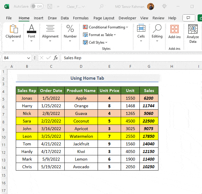
Hello DIALLO,
Thanks for your appreciation. I can get the problem you are facing with your worksheet.
Here, we have a dummy dataset in our hands to replicate your problem. It’s a Sales Report of a particular grocery store.
From the above dataset, we can clearly notice that there is a total of two sales that are greater than $15000, and others are less than this amount.
Now, we’ll show how you would do it in your workbook.
• At the very beginning, select cells in the B5:D14 range.
• After that, go to the Home tab.
• Then, click on the Conditional Formatting drop-down on the Styles group.
• Next, select New Rule from the list.
In the New Formatting Rule dialog box,
• At first, choose Use a formula to determine which cells to format under the Select a Rule Type section.
• Secondly, write down the following in the Format values where this formula is true box.
=D5<=15000• Thirdly, click on the Format button.
The Format Cells dialog box appears.
• Firstly, move to the Fill tab.
• Following this, select Red as Background Color.
• Later, click OK.
• Also, click OK in the New Formatting Rule dialog box.
Immediately, it shows us faulty formatting which we don’t want.
So, how can we fix it? Don’t worry! We just have to edit the formula.
To do this,
• Initially, proceed to the Home tab.
• Then, click on the Conditional Formatting drop-down.
• From the drop-down list, select Manage Rules.
Suddenly, it opens the Conditional Formatting Rules Manager.
• Primarily, select This Worksheet in the Show formatting rule for box.
• Secondarily, select the rule.
• Thirdly, click on Edit Rule.
• Change the formula a little bit. Just add a ($) sign before D5.
• Lastly, click OK.
• Again, click OK.
Now, you can see the correct formatting according to your preference.
That’s all from me on this. Keep the good vibes. You can follow our website Exceldemy, a one-stop Excel solution provider to explore more. Happy Excelling☕…..
Hello,
First of all, download the Practice Workbook for better understanding.
I think you’ve talked about the following phenomena. Let’s see the following image.
Now, you want to match the items in Column 2020 with the items in Column 2019.
For this, copy the cells in the B5:B12 range.
Then, paste them in the E5:E12 range.
After that, go to cell F5 and enter the following formula.
=IF(COUNTIF(C5:C12,B5:B12)>0,B5:B12,"")As usual, press ENTER.
Note: It’s an array formula. If you are using Microsoft Excel 365 then you can easily run the formula by pressing the ENTER key. Otherwise, you have to tap the CTRL+SHIFT+ENTER keys simultaneously to make the formula work.
Hope that will work for you. Follow our blog Exceldemy to learn more about Excel.
Hello ROMA,
Sorry for being late. And we love to solve our user’s problems.
First of all, download the Practice Workbook for your own convenience.
• At the very beginning, we’ve made a relevant dataset for your problem.
• Then, make a new row in Row 9 with the heading Total Monthly Sales. Also, a new column Total Sales in Column F.
• Later, select cell C9 and enter the formula below.
=SUM(C5:C8)• Next, press ENTER.
• Alternatively, press ALT+= on the keyboard as a shortcut to do the same task.
• Now, get the cursor to the bottom-right corner of cell C9; instantly, it will look like a plus (+) sign. Actually, it’s the Fill Handle tool.
• Thus, drag it to the right corner of cell E9.
Therefore, we get the desired results in other cells too.
• Similarly, go to cell F5 and paste the following formula.
=SUM(C5:E5)• As usual, press ENTER.
Currently, we’ll insert the chart.
• Firstly, go to the Insert tab.
• Secondly, click on Insert Column or Bar Chart dropdown on the Charts group.
• Thirdly, select 2-D Clustered Column from the available options.
As a result, we can see a blank chart on the worksheet.
• Then, right-click anywhere on the chart area.
• It opens a context menu. Hence, choose Select Data from the options.
Immediately, the Select Data Source dialog box opens.
• Here, click on the Add button under the Legend Entries (Series) section.
Instantly, the Edit Series input box appears.
• Then, give the Series name as Monthly Sales.
• In the box of Series values, give the reference of the C9:E9 range.
• After that, click OK.
• Thenceforth, click on the Edit button under the Horizontal (Category) Axis Labels.
• Following this, give the reference of the C4:E4 range in the Axis label range box.
• After that, click OK.
It returns us to the Select Data Source dialog box again.
• Next, press the OK button.
Simply, a column chart will be visible on the worksheet. It includes the month-wise sales amount.
• Hereafter, add Axis Titles and Legend to the chart using the Add Chart Element option.
Now, we’ll create the second chart as per your question.
• Similarly, insert another blank chart and open the Select Data Source dialog box.
• Then, click on Add.
• Then, in the Edit Series dialog box, do the following as in the image below.
• Also, change the Horizontal Axis Labels like before.
• After that, click OK.
Here is the desired chart of employee-wise total sales.
• Bring some edits to the chart to make it more appealing.
Hello DEANNA,
First of all, many many thanks for your appreciation. At the end of the day, these kinds of words motivate us a lot. Now, get back to your query.
For your convenience, download this practice workbook.
Firstly, we’ve created a dataset as per your description. We’ve constructed an imaginary Weekly Sales Report of your company. Let’s see the following picture.
Now, we’ll find out how many sales reps cannot cross the Sales Amount of $350 in a week.
At first, go to cell D11 and enter the following formula into the cell.
=COUNTIF(D5:D9,"<350")Secondly, press the ENTER key.
Here, we can see that Excel returns 2 as result. Because two employees made sales amount below $350 which are Person 2 and Person 5. We think you wanted to know about this part.
As a bonus, we’ll teach you one more trick. You can get a more specific answer with this. Guess, if you wanted to know how many sales reps made sales amount below $350 in a specific zone. Let’s say, in the West zone. Obviously, you can crack this too.
Firstly, select cell D11 and write down the formula below.
=COUNTIFS(D5:D9,"<350",C5:C9,"West")As usual, tap ENTER.
The result is 1 because there is only one Sales Rep in the West zone with a Sales Amount less than $350 who is Person 2.
To explore more about Excel, please visit our website Exceldemy: One-stop Excel solution provider…
Hello Dave,
Thanks for your humble appearance. But we always welcome informing us about your concerns. Now, without further delay, let’s dive into the problem.
At first, download the Practice Workbook for your own convenience.
From your example above, I’ve created a dataset. Let’s look at the image below for a better understanding.
• To solve the problem, firstly, we are creating a new column named Helper Column to Get Date Only. Also, created a final output range in cell D14.
• Secondly, select cell D7 and enter the following formula.
=DATE(YEAR(B7),MONTH(B7),DAY(B7))This formula filters out the date only from the date and time in cell B7.
• Then, press the ENTER key.
• After that, use the Fill Handle tool to get results in the remaining cells.
• Thirdly, go to cell D14 and paste the formula below.
=MAX(IF(D7:D12=D4,B7:C12))We used the MAX and IF functions in the formula above. Using the IF function, we inserted a logical test that checks if the dates in the D7:D12 range equals to the date in cell D4. If the result is TRUE, then it displays an array of corresponding dates and times in the B7:C12 range. Then, the MAX function gets the maximum value among them.
• As usual, press ENTER.
Currently, it’s showing the time in General format. So, we’ve to change the cell formatting.
• To do this, press CTRL+1 to open the Format Cells dialog box.
• In the Number tab, select Time format as Category.
• Then, choose the formatting Type as shown in the picture below.
• Lastly, click OK.
Finally, we got our desired output format. And the result is correct also.
That’s all about it. If you find any difficulty regarding this example or any other problems related to Excel, feel free to contact us. You can also follow our Exceldemy blog for the most detailed solutions to any problems in Excel.
Hello MOHAMAD,
Thanks for your valuable comment. We always expect such positive feedback from our users.
As you said, here we’ve shown the simple exponential method only. The main reason for this is that we didn’t only want to emphasize exponential smoothing; rather we wanted to cover all conceivable methods of data smoothing. If so happened the article would then be extremely lengthy.
But you can find triple exponential smoothing widely called the Holt-Winters Exponential Smoothing on our website also. This method is very much adaptable for data with seasonal patterns.
Thanks Again.
Hello Siam A,
In the first place, thanks for your this kind of support. This is what motivates us to move forward.
Now, let’s get back to your problem. Here, I’ve created a dataset from the information you provided in the comment. Get a look at the dataset first.
Then, in cell F5, we’ll fetch the minimum value of A. As the dataset is small enough, we can see that the min value of A is 180. Let’s see if we get the same value with our formula.
Firstly, select cell F5 and write down the following formula into the cell.
=IF(B5:B13="A",C5:C13)Then, press ENTER.
Here, we got an array in Column F. If the corresponding cell in Column B holds A, then in the cell in Column F, we get the consecutive value of A. Otherwise, it returns FALSE.
After that, apply the MIN function with the formula to find the minimum value from the array.
So, again, go to cell F5 and edit the formula. Now, it’ll look like the one below.
=MIN(IF(B5:B13="A",C5:C13))Thus, press ENTER.
Finally, we’ve got the min value of A.
Similarly, we can obtain the min value of B. Just, select cell F6 and paste the following formula.
=MIN(IF(B5:B13="B",C5:C13))Then, press the ENTER key.
Corresponding, get the minimum of value of C. Just write down C inside the double quote marks of the formula.
Note: The problem with VLOOKUP is that it always get the first value for the lookup value. For example, using the VLOOKUP function to get the minimum value of B, you’ll always receive 360. Because, after retrieving the value 360 it doesn’t go down further. But the correct result should be 160.
You can download the practice workbook for better understanding.
Hope you will find the solution helpful. Don’t forget to subscribe to our website Exceldemy: One-stop Excel sotuion provider…
If your workbook is shared, anyone who has Write privileges can clear the read-only status.
Follow Method 1. Paste Link Option. Just make a little bit of change. Select Paste Specials > Other Paste Options > Linked Picture.
In this situation, you can use an easy alternative. Try using:
=COUNTA(UNIQUE(date range))
The above formula can easily count the unique date values.