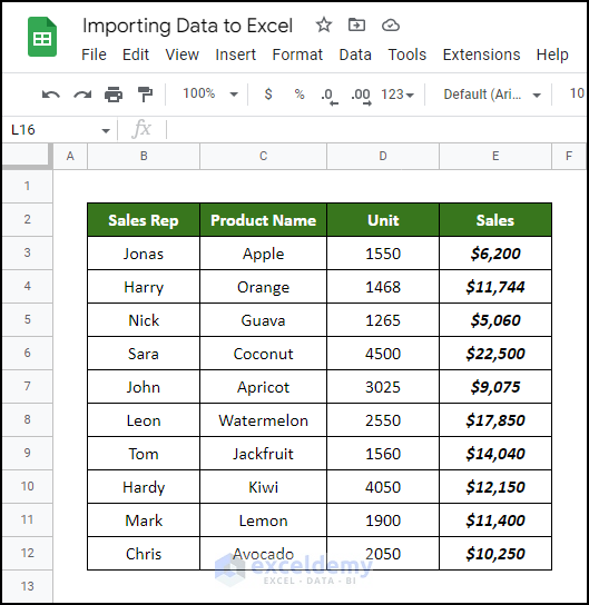
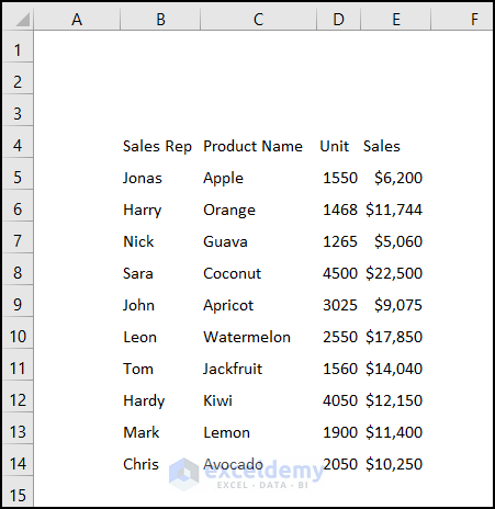
How to Import Data from Google Sheets to Excel Using VBA

The name of the sheet is Importing Data to Excel. The dataset includes Sales Rep, Product Name, Unit, and Sales.

import data from google sheets to excel vba

Step 1 – Change the Privacy of Google Sheets

Steps:

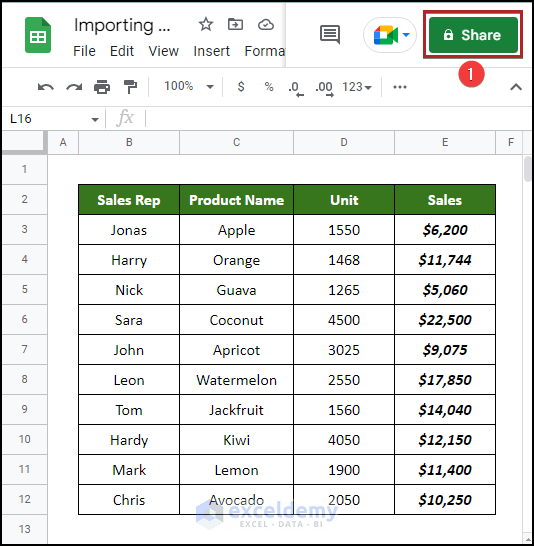
Click Share.

Change Privacy of Google Sheets

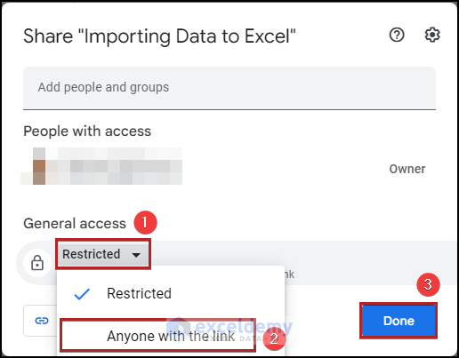
The Share “Importing Data to Excel” dialog box is displayed.

Click the drop-down arrow in General access.
Select Anyone with the link.
Click Done.

Making the Google Sheets Accessible for everyone

Step 2 – Enter the VBA Code to Import Data to Excel

Steps:

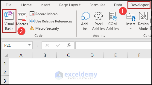
Open a new workbook.
Go to the Developer tab.
Click Visual Basic in Code.

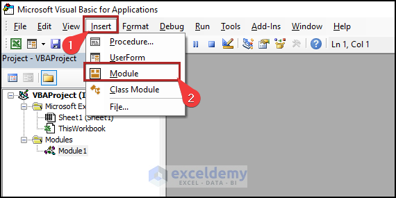
Insert VBA Code to Import Data to Excel

In the Microsoft Visual Basic for Applications window:

Go to the Insert tab.
Select Module.

Inserting Code Module

Enter the following code in the module.

Sub Import_Sheets_to_Excel()
Dim QRT As QueryTable, ul As String, ky As String
If ActiveSheet.QueryTables.Count > 0 Then ActiveSheet.QueryTables(1).Delete
ActiveSheet.Cells.Clear
ky = "1slumgR5et-cG7Er-9udweCSthufb7xYdsmoP9H2AOFs"
ul = "https://spreadsheets.google.com/tq?tqx=out:html&key=" & ky
Set QRT = ActiveSheet.QueryTables.Add(Connection:="URL;" & ul, _
Destination:=Range("$A$4"))
With QRT
.WebSelectionType = xlAllTables
.WebFormatting = xlWebFormattingNone
.Refresh
End With
End Sub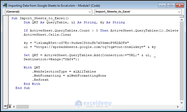

VBA Code to import data from google sheets to excel

Code Breakdown

The different variables are declared.
The If logical statement is added to clear tables or data in the worksheet.
The ky variable is set: it’s the Google spreadsheet key. You can obtain this key from the sheet’s sharing link on the address bar. Locate it after “/d/” and before the next forward slash. See the address below:

https://docs.google.com/spreadsheets/d/1slumgR5et-cG7Er-9udweCSthufb7xYdsmoP9H2AOFs/edit#gid=0

The bold part is the spreadsheet key.

Set the output of the Google spreadsheet data as an HTML table with a modified URL:

“https://spreadsheets.google.com/tq?tqx=out:html&key=” & ky

The query is added to the Excel sheet and the destination range is defined: A4.

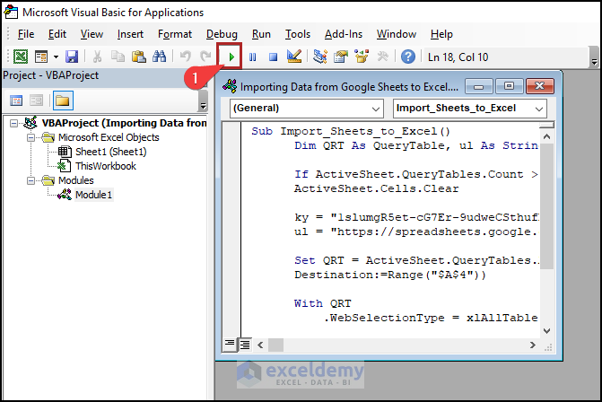
Run the code by clicking the play button on the ribbon.

Run the VBA Code to import data from google sheets to excel

Go back to the worksheet: Sheet1.

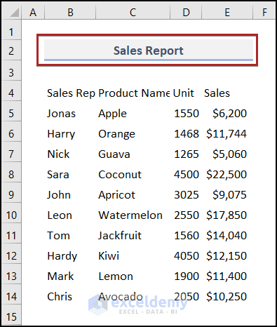
Excel is getting the data from an external source.

Getting Data from Google Sheets to Excel

This is the output.

Extracted Data from Google Sheets

Step 3 – Apply Formatting to the Dataset

Steps:

Create a heading in B2. It’s formatted in Heading 2 Cell Style.

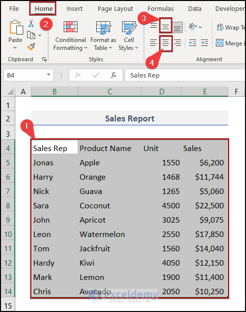
Apply Formatting to Dataset to Make It Engage

Select B4:E14.
Go to the Home tab.
Click the Middle Align icon and the Center icon in Alignment.

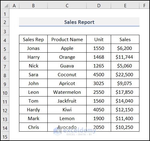
Applying Center and Middle Alignment

Set All Borders.

This is the output.

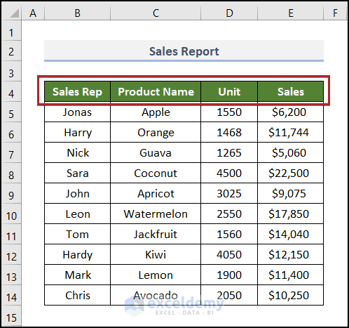
Applying All Borders to the dataset

Select the headings in B4:E4 and make them Bold. Change the Fill Color and Font Color.

Apply Formatting to Imported data from Google Sheets to Excel to Make It Engage

Download Practice Workbook

Download the Excel workbook.

Importing Data From Google Sheets to Excel.xlsm

<< Go Back to Import Google Sheets to Excel | Importing Data in Excel | Learn Excel

Get FREE Advanced Excel Exercises with Solutions!

Sub ImportDataFromGoogleSheets() 'Set the URL of the Google Sheets document Dim googleSheetsURL As String googleSheetsURL = "https://docs.google.com/spreadsheets/d/XXXXXXXXXXXXXXXXXXXXXXXXXXXXXXXXXXXXXXXXXXXX/edit#gid=YYYYYYYYYY" 'Set the name of the sheet containing the data you want to import Dim sheetName As String sheetName = "Sheet2" 'Set the target range where you want to paste the imported data Dim targetRange As Range Set targetRange = ThisWorkbook.Worksheets("Sheet1").Range("A1") 'Define the source range of the data in the Google Sheets document Dim sourceRange As Range With CreateObject("MSXML2.XMLHTTP") .Open "GET", googleSheetsURL, False .send Dim responseText As String responseText = .responseText Dim startIndex As Long startIndex = InStr(1, responseText, sheetName & "!A1") If startIndex > 0 Then Dim endIndex As Long endIndex = InStr(startIndex, responseText, "class=""") - 1 If endIndex > startIndex Then Dim rangeAddress As String rangeAddress = Mid(responseText, startIndex, endIndex - startIndex) rangeAddress = Replace(rangeAddress, "'", "") rangeAddress = Replace(rangeAddress, "!", ":") Set sourceRange = Range(rangeAddress) End If End If End With 'Copy the data from the source range to the clipboard sourceRange.Copy 'Clear the target range to ensure that no existing data interferes with the import targetRange.CurrentRegion.ClearContents 'Paste the data from the clipboard into the target range targetRange.PasteSpecial xlPasteValues End Sub

' Load the Google API client library Private Sub LoadGoogleAPI() Dim objHTTP As Object Set objHTTP = CreateObject("MSXML2.XMLHTTP") objHTTP.Open "GET", "https://developers.google.com/oauthplayground/assets/js/library.js", False objHTTP.send Dim html As Object Set html = CreateObject("htmlfile") html.body.innerHTML = objHTTP.responseText Dim script As Object Set script = html.createElement("script") script.Language = "javascript" script.Text = "function DoNothing() {}" html.appendChild script Set google = html.parentWindow End Sub ' Authenticate to Google Sheets Private Sub AuthenticateToGoogle() Dim CLIENT_ID As String Dim CLIENT_SECRET As String Dim REFRESH_TOKEN As String CLIENT_ID = "your_client_id_here" CLIENT_SECRET = "your_client_secret_here" REFRESH_TOKEN = "your_refresh_token_here" ' Load the Google API client library LoadGoogleAPI ' Authenticate with Google google.gapi.auth.authorize Array("https://www.googleapis.com/auth/spreadsheets"), CLIENT_ID, CLIENT_SECRET, REFRESH_TOKEN ' Get the access token access_token = google.gapi.auth.getToken().access_token End Sub ' Upload data to Google Sheets Private Sub UploadDataToGoogleSheets() ' Authenticate with Google AuthenticateToGoogle ' Define the range of data to upload Dim range As String range = "Sheet1!A1:D4" ' Change this to the range of your data ' Get the spreadsheet ID Dim spreadsheet_id As String spreadsheet_id = "your_spreadsheet_id_here" ' Define the data to upload Dim data As Variant data = Range(range).Value ' Upload the data to Google Sheets Dim url As String url = "https://sheets.googleapis.com/v4/spreadsheets/" & spreadsheet_id & "/values/" & range & "?valueInputOption=USER_ENTERED" Dim xmlhttp As Object Set xmlhttp = CreateObject("MSXML2.XMLHTTP") xmlhttp.Open "PUT", url, False xmlhttp.setRequestHeader "Authorization", "Bearer " & access_token xmlhttp.setRequestHeader "Content-Type", "application/json" Dim json As String json = "{""values"": " & WorksheetFunction.Transpose(WorksheetFunction.Transpose(JsonConverter.ConvertToJson(data))) & "}" xmlhttp.send json End Sub

Sub Import_Sheets_to_Excel() Dim QRT As QueryTable, ul As String, ky As String If ActiveSheet.QueryTables.Count > 0 Then ActiveSheet.QueryTables(1).Delete ActiveSheet.Cells.Clear ky = "1slumgR5et-cG7Er-9udweCSthufb7xYdsmoP9H2AOFs" ul = "https://spreadsheets.google.com/tq?tqx=out:html&key=" & ky & "&range=A1:E10" Set QRT = ActiveSheet.QueryTables.Add(Connection:="URL;" & ul, _ Destination:=Range("$A$4")) With QRT .WebSelectionType = xlAllTables .WebFormatting = xlWebFormattingNone .Refresh End With End Sub

Sub Import_Sheets_to_Excel() Dim QRT As QueryTable, ul As String ' Enter the URL of your online Excel ul = "https://1drv.ms/x/s!AhXZPAkXAN3YmQlrC8RvdAWRh31H?e=XwaZc4" If ActiveSheet.QueryTables.Count > 0 Then ActiveSheet.QueryTables(1).Delete ActiveSheet.Cells.Clear Set QRT = ActiveSheet.QueryTables.Add(Connection:="URL;" & ul, _ Destination:=Range("$A$4")) With QRT .WebSelectionType = xlAllTables .WebFormatting = xlWebFormattingNone .Refresh End With End Sub

Sub ImportDataFromExcel365() Dim sourceWorkbook As Workbook Dim sourceSheet As Worksheet Dim sourceRange As String Set sourceWorkbook = Workbooks.Open("https://1drv.ms/x/s!AiLbipRfCPXPkWiuZTaSCmdP1XKp?e=5rmfGX") Set sourceSheet = sourceWorkbook.Sheets("Sheet1") sourceRange = "A1:B10" Dim destinationWorkbook As Workbook Dim destinationSheet As Worksheet Dim destinationCell As Range Set destinationWorkbook = ThisWorkbook Set destinationSheet = destinationWorkbook.Sheets("DestinationSheet") Set destinationCell = destinationSheet.Range("A1") With destinationWorkbook.Connections.Add2("Excel365 Query", "", sourceRange, "Excel365", 6) .OLEDBConnection.BackgroundQuery = False .OLEDBConnection.RefreshOnFileOpen = False .Refresh End With sourceSheet.UsedRange.Copy destinationCell End Sub

14 Comments

Obot Feb 13, 2023 at 5:30 PM

How do I import the data from other sheets other than the sheet1 of googlesheet?

Sabrina Ayon Feb 15, 2023 at 12:45 PM

Hello, OBOT!
Thanks for your comment!
To import data from a specific sheet (e.g., “Sheet2“) of a Google Sheets document to Excel using VBA, you can use the following code:

To use this code, you need to replace the googleSheetsURL variable with the URL of the Google Sheets document containing the data you want to import and replace the sheetName variable with the name of the sheet containing the data you want to import (in this example, “Sheet2“). You also need to set the targetRange variable to specify the cell or range where you want to paste the imported data (in this example, cell A1 of the Sheet1 worksheet).

The code uses the MSXML2.XMLHTTP object to send an HTTP request to the Google Sheets document, and parses the HTML response to identify the range of cells corresponding to the specified sheet name. It then copies the data from the identified range to the clipboard, clears the target range to ensure that no existing data interferes with the import, and pastes the data from the clipboard into the target range.

Hope this will help you!
Good Luck!

Regards,
Sabrina Ayon
Author, ExcelDemy.

Reza Mar 12, 2023 at 1:14 PM

Hello dear
Thanks you…
Is it possible to write a VBA program to upload data from an Excel file directly to Google Sheets?
- Reply
  Shahriar Abrar Rafid Mar 15, 2023 at 4:22 PM
  Hello REZA,
  Thanks for commenting and asking your valuable question. Actually, it’s quite costly to do it with VBA. Because of this, you have to enable the Google Sheets API, and quite expensive. So I wouldn’t suggest it.
  Rather, you can use Google Drive or the Import feature of Google Sheets to do this task easily. You can follow this linked article on our website to get the whole idea.
  Anyway, if you want to do it with VBA, you can follow this lengthy process:
  - First, you have to enable the Google Sheets API for your Google account and create a project in the Google Developers Console. Here are the steps to enable the Google Sheets API and create a project in the Google Developers Console:
  - Go to the Google Cloud Console website (https://console.cloud.google.com/).
  - If you don’t have a Google Cloud account, sign up for a free trial or create a new account.
  - Once you’re signed in to the Google Cloud Console, create a new project by clicking the “Select a project” dropdown menu in the top navigation bar and clicking “New Project“.
  - Give your project a name and click “Create“.
  - In the left-hand navigation menu, click “APIs & Services” and then click “Dashboard“.
  - Click the “+ ENABLE APIS AND SERVICES” button at the top of the page.
  - In the search bar, type “Google Sheets API” and click on the result.
  - Click the “ENABLE” button to enable the Google Sheets API for your project.
  - Next, you need to create a set of credentials to authenticate your VBA program with your Google account. In the left-hand navigation menu, click “Credentials“.
  - Click the “Create credentials” dropdown menu and select “OAuth client ID“.
  - Select “Desktop app” as the application type, give your client ID a name, and click “Create“.
  - In the “OAuth client created” dialog box, click “OK“.
  - Click on the name of the client ID you just created to download the client secret file.
  - Rename the downloaded file to “client_secret.json” and save it in a secure location on your computer.
  - Finally, authorize the API scopes for your Google account by clicking the “Configure consent screen” button on the “Credentials” page and following the prompts to enter your app details and authorized scopes.
  - After that, Create a Google Sheets spreadsheet and give it a name.
  - In VBA, create a reference to the Google API client library and authenticate to your Google account. Here is a sample VBA code to do it:
```
' Load the Google API client library
Private Sub LoadGoogleAPI()
    Dim objHTTP As Object
    Set objHTTP = CreateObject("MSXML2.XMLHTTP")
    objHTTP.Open "GET", "https://developers.google.com/oauthplayground/assets/js/library.js", False
    objHTTP.send
    Dim html As Object
    Set html = CreateObject("htmlfile")
    html.body.innerHTML = objHTTP.responseText
    Dim script As Object
    Set script = html.createElement("script")
    script.Language = "javascript"
    script.Text = "function DoNothing() {}"
    html.appendChild script
    Set google = html.parentWindow
End Sub

' Authenticate to Google Sheets
Private Sub AuthenticateToGoogle()
    Dim CLIENT_ID As String
    Dim CLIENT_SECRET As String
    Dim REFRESH_TOKEN As String
    CLIENT_ID = "your_client_id_here"
    CLIENT_SECRET = "your_client_secret_here"
    REFRESH_TOKEN = "your_refresh_token_here"
    
    ' Load the Google API client library
    LoadGoogleAPI
    
    ' Authenticate with Google
    google.gapi.auth.authorize Array("https://www.googleapis.com/auth/spreadsheets"), CLIENT_ID, CLIENT_SECRET, REFRESH_TOKEN
    
    ' Get the access token
    access_token = google.gapi.auth.getToken().access_token
End Sub

' Upload data to Google Sheets
Private Sub UploadDataToGoogleSheets()
    ' Authenticate with Google
    AuthenticateToGoogle
    
    ' Define the range of data to upload
    Dim range As String
    range = "Sheet1!A1:D4" ' Change this to the range of your data
    
    ' Get the spreadsheet ID
    Dim spreadsheet_id As String
    spreadsheet_id = "your_spreadsheet_id_here"
    
    ' Define the data to upload
    Dim data As Variant
    data = Range(range).Value
    
    ' Upload the data to Google Sheets
    Dim url As String
    url = "https://sheets.googleapis.com/v4/spreadsheets/" & spreadsheet_id & "/values/" & range & "?valueInputOption=USER_ENTERED"
    Dim xmlhttp As Object
    Set xmlhttp = CreateObject("MSXML2.XMLHTTP")
    xmlhttp.Open "PUT", url, False
    xmlhttp.setRequestHeader "Authorization", "Bearer " & access_token
    xmlhttp.setRequestHeader "Content-Type", "application/json"
    Dim json As String
    json = "{""values"": " & WorksheetFunction.Transpose(WorksheetFunction.Transpose(JsonConverter.ConvertToJson(data))) & "}"
    xmlhttp.send json
End Sub
```
  Just make sure to change specific things in your own code. Hope this could help you. Again, thanks to you.
  
  Regards
  SHAHRIAR ABRAR RAFID
  Team ExcelDemy
  - Reply
    Robert Apr 30, 2023 at 9:44 PM
    
    this doesnt work
    - Shahriar Abrar Rafid May 2, 2023 at 11:40 AM
      
      Hello ROBERT,
      Do you have Google API? I think the code works. But if it doesn’t work for you, you can use the simple Import feature which I mentioned in the previous reply.
      Even if you want to do it with VBA, you can do it through Google Forms. This process doesn’t require the API key.
      If you have further queries, you can comment below. Thanks for your feedback.
      Regards
      SHAHRIAR ABRAR RAFID
      Team ExcelDemy
Georgi Mar 16, 2023 at 9:57 PM

Hello – this is amazing information. I ahve been strugling to get it to work for ages. Can i shoose which rage to extract from the google sheet?
- Reply
  Shahriar Abrar Rafid Mar 21, 2023 at 11:02 AM
  Hello GEORGI,
  Thanks for appreciating our work. We are also happy to release you from prolonged suffering. Now, get back to your query.
  Sure, you can alter the “Destination” parameter of the “QueryTables.Add” method in your script to specify a specific range to extract from the Google sheet.
  For instance, you could change the code such that it retrieves data from cells A1 to E10 of the sheet:
```
Sub Import_Sheets_to_Excel()

    Dim QRT As QueryTable, ul As String, ky As String
    If ActiveSheet.QueryTables.Count > 0 Then ActiveSheet.QueryTables(1).Delete
    ActiveSheet.Cells.Clear
    ky = "1slumgR5et-cG7Er-9udweCSthufb7xYdsmoP9H2AOFs"
    ul = "https://spreadsheets.google.com/tq?tqx=out:html&key=" & ky & "&range=A1:E10"
    Set QRT = ActiveSheet.QueryTables.Add(Connection:="URL;" & ul, _
    Destination:=Range("$A$4"))
    With QRT
        .WebSelectionType = xlAllTables
        .WebFormatting = xlWebFormattingNone
        .Refresh
    End With

End Sub
```
  The “ul” variable in this modified code has the addition “&range=A1:E10” to identify the range to extract from. Also, the starting cell where the extracted data will be stored is specified by the “Destination” parameter in the “QueryTables.Add” method, which is set to “$A$4“.
  I hope this helps. I wanted to personally invite you to check out our new Excel-related forum. We’ve created a space for Excel enthusiasts like us to share tips, tricks, and ideas, as well as to ask and answer questions about using Excel. We’re a growing community of Excel users, and we’d love to have you join us!
  Here’s the link to our forum: ExcelDemy Forum
  
  Regards,
  SHAHRIAR ABRAR RAFID
  Team ExcelDemy
Huongpt Nov 8, 2023 at 12:11 PM

Thank you!

I want to get data from Excel 365 (web) to Excel by VBA (the same)?
- Reply
  Yousuf Khan Nov 9, 2023 at 12:37 PM
  Hello HUONGPT,
  
  Thanks for sharing your experience with us!
  
  The code shared in this article is designed to import data from a Google Sheets web version to an Excel offline version. It uses a Google Sheets key to access the data.
  
  To modify this code for Microsoft 365 Excel online version, you would need to adapt it to use the appropriate URL for your Microsoft 365 Excel file. Microsoft 365 Excel doesn’t use a key like Google Sheets, but rather the URL of the shared document. Use the below VBA code instead:
```
Sub Import_Sheets_to_Excel()
    Dim QRT As QueryTable, ul As String

    ' Enter the URL of your online Excel
    ul = "https://1drv.ms/x/s!AhXZPAkXAN3YmQlrC8RvdAWRh31H?e=XwaZc4"

    If ActiveSheet.QueryTables.Count > 0 Then ActiveSheet.QueryTables(1).Delete
    ActiveSheet.Cells.Clear

    Set QRT = ActiveSheet.QueryTables.Add(Connection:="URL;" & ul, _
        Destination:=Range("$A$4"))

    With QRT
        .WebSelectionType = xlAllTables
        .WebFormatting = xlWebFormattingNone
        .Refresh
    End With
End Sub
```
  You can also import data from online Excel without VBA quite easily. Here is how:
  
  1. When you open your Online Excel file there is an option called Edit.
  2. Select Edit in Online Excel >> then it will open in Desktop Excel.
  3. Now, you will have all the options. It is as easy as it sounds!
  
  Hope these suggestions help. Keep excelling.
  
  Regards,
  Yousuf Khan Shovon

HUONGPT Nov 26, 2023 at 9:15 PM

Thank you!

But the code not work with my ULR, get message box “This Web Query returned no data…”. I get URL from “Share” link in Excel web.

Lutfor Rahman Shimanto Nov 27, 2023 at 5:18 PM

Hello HUONGPT

Thanks for sharing your problem. You want to get data from Excel 365 (WEB) to a local Excel application. Fencing data from Excel 365 (WEB) is different from importing data from Google Sheets. I am presenting an Excel VBA sub-procedure. However, you must have valid Windows Security credentials on your own.

Excel VBA Sub-procedure:

After Running the code, the Windows Security dialog box will appear => Next, insert the intended username and password => Hit OK.

Hopefully, the idea will help you. Good luck!

Regards
Lutfor Rahman Shimanto

Huongpt Dec 4, 2023 at 3:07 PM

Thank for support!
- Reply
  Shamima Sultana Dec 5, 2023 at 9:36 AM
  
  Hello Huongpt,
  
  You are welcome.
  
  Regards
  ExcelDemy

How to Import Data from Google Sheets to Excel Using VBA – 3 Steps

Step 1 – Change the Privacy of Google Sheets

Step 2 – Enter the VBA Code to Import Data to Excel

Step 3 – Apply Formatting to the Dataset

Related Articles

Leave a reply Cancel reply