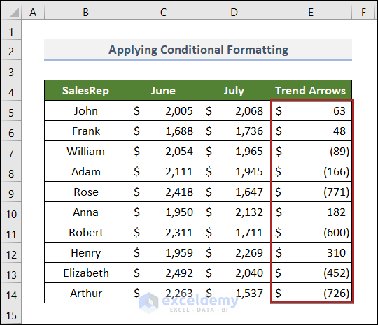
This dataset includes SalesRep’s name, and sales for June and July in columns B, C, and D.
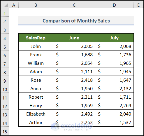
Trend arrows can show the increase or decrease in sales.
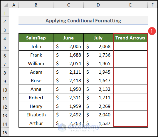
Method 1 – Applying the Conditional Formatting
- Insert a new column with the heading Trend Arrows: Column E.
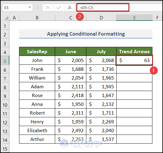
- Select E5 and enter the following formula.
=D5-C5
C5 and D5 represent John’s sales in June and July.
- Press ENTER.
- Place the cursor at the bottom-right corner of E5. The plus (+) sign is the Fill Handle tool.
- Double-click it.
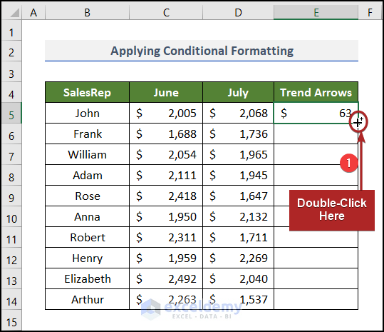
All other cells in E5:E14 will automatically be filled.
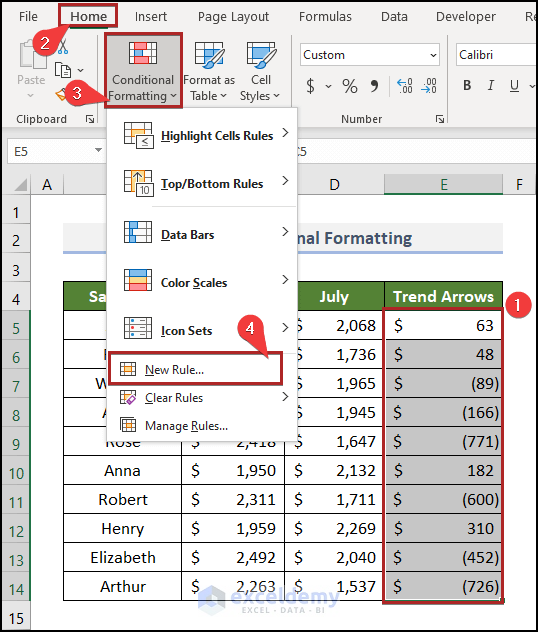
- Select E5:E14.
- Go to the Home tab.
- Select Conditional Formatting.
- Choose New Rule.
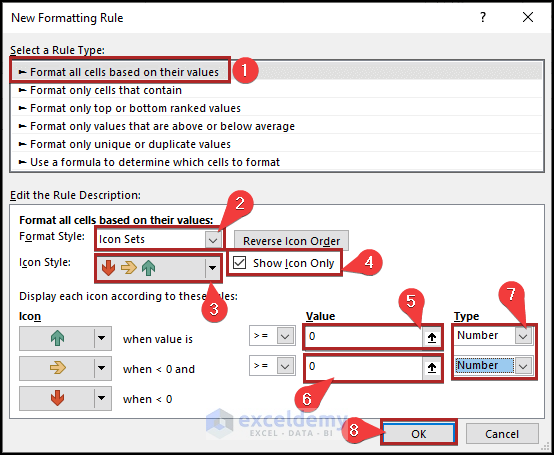
In the New Formatting Rule dialog box:
- In Select a Rule Type, choose Format all cells based on their values.
- Go to Edit the Rule Description.
- Select Icon Sets as Format Style.
- In Icon Style, choose 3 Arrows (Colored).
- Check Show Icon Only.
- Enter 0, in Value.
- Change Type to Number.
- Click OK.
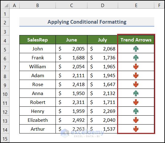
Column E is displayed with trend arrows.
Read More: How to Add Trend Arrows in Excel
Method 2- Using Different Symbols
Steps:
- Insert a new column like in Method 1.
- Select B16:C16.
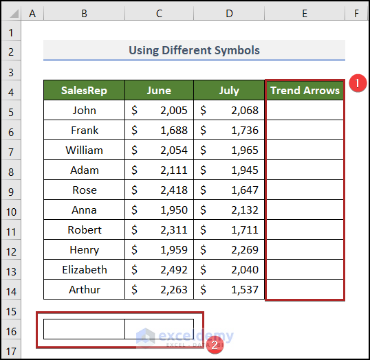
- Go to B16.
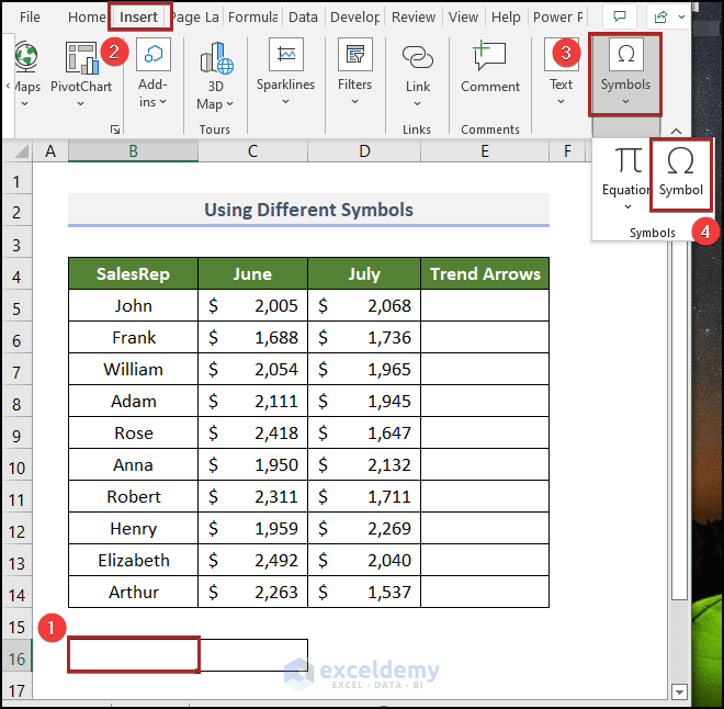
- In the Insert tab, click Symbols.
- Select Symbol.
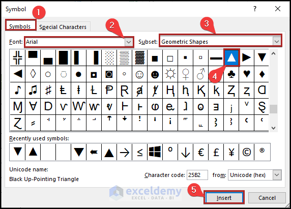
In the Symbol wizard:
- Select Symbols.
- Choose Arial, in Font.
- In Subset, choose Geometric Shapes.
- Select Black Up-Pointing Triangle.
- Click Insert.
- Insert the Black Down-Pointing Triangle in C16.
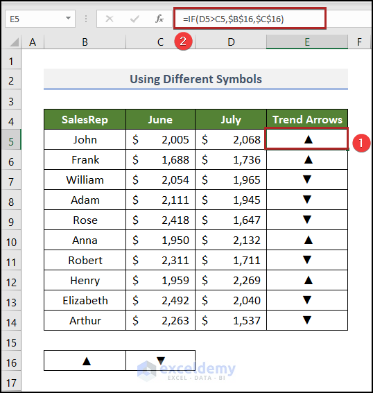
- Go to cell E5 and enter the following formula.
=IF(D5>C5,$B$16,$C$16)
C5 and D5 are John’s sales for June and July. B16 represents the cell reference of an up-pointing triangle. C16 is the reference for the down-pointing triangle. The IF function performs a logical test: the value in D5 is greater than the value in C5. If this is TRUE, E5 will get the value of B16. Otherwise, it will hold the value of C16.
Here, the value of D5 is greater than the value of C5. So, the up-pointing triangle is displayed in E5.
- Press ENTER.
Read More: How to Add Up and Down Arrows in Excel
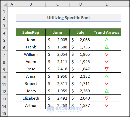
Method 3 – Utilizing a Specific Font
Steps:
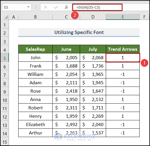
- Go to E5 and enter the formula below.
=SIGN(D5-C5)
The SIGN function returns the sign of a number. It returns 1 for positive numbers. For negative values, -1. Otherwise, 0.
- Press ENTER.
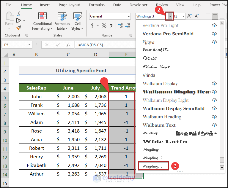
- Select all cells in E5:E14.
- Click Font.
- Select Windings 3.
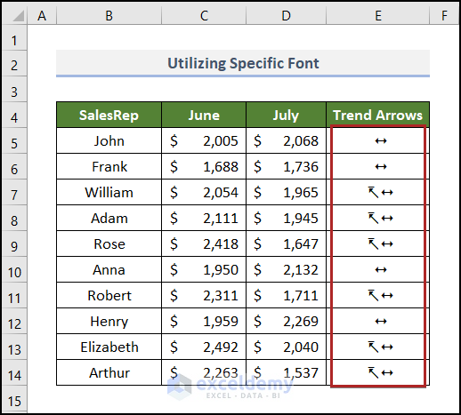
This is the output.
- Select E5:E14.
- Press CTRL+ 1.
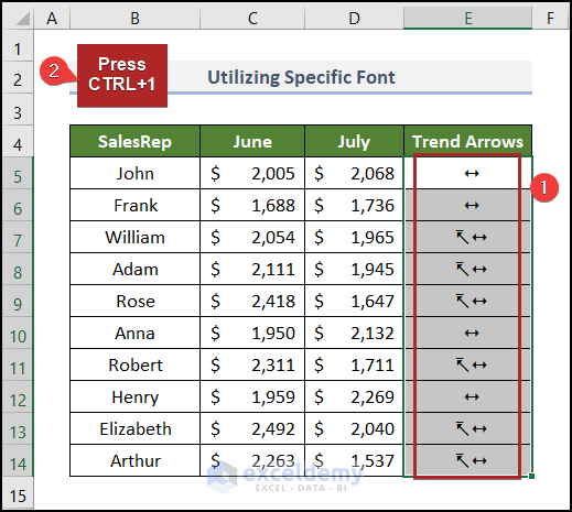
In Format Cells:
- Go to the Number tab.
- In Category, select Custom.
- In Type, enter the following.
[Green]\r;[Red]\s;
- Click OK.
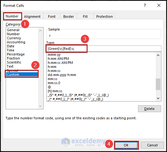
The trend arrows are displayed.
Read More: Up and Down Arrows in Excel Using Conditional Formatting
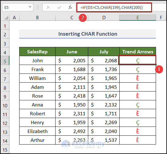
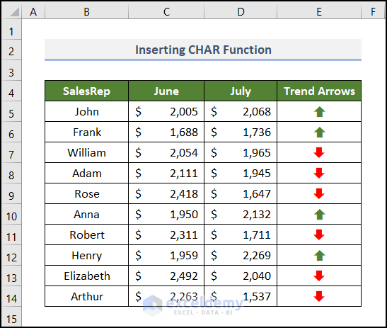
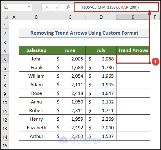
Method 4 – Inserting the CHAR Function
Steps:
- Select E5 and enter the following formula.
=IF(D5>C5,CHAR(199),CHAR(200))
This formula is similar to the one used in Method 2.
- Press ENTER.
- Select E5:E14.
- Go to the Home tab.
- Click Font.
- Select Windings 3.
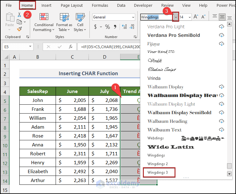
Symbols change into trend arrows.
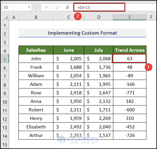
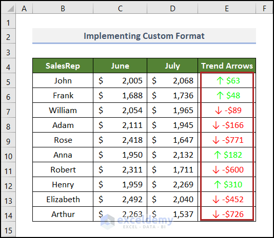
Method 5 – Using the Custom Format
Steps:
- Select E5 and enter following formula in the Formula Bar.
=D5-C5
- Press ENTER.
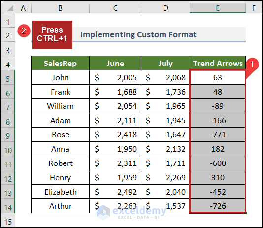
- Select the Trend Arrows column without the heading.
- Press CTRL+1 to open the Format Cells dialog box.
- Select Custom in Category.
- Enter the following in Type.
[Green] ↑ $0;[Red] ↓ -$0
- Click OK.
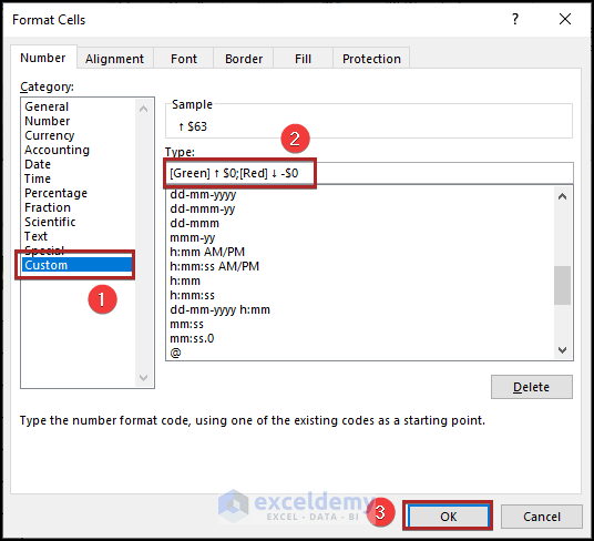
Trend arrows are displayed in Column E.
Read More: Double Headed Arrow in Excel
How to Remove Trend Arrows
1. Removing Trend Arrows by Clearing the Rule
In Method 1, trend arrows were inserted by applying the Conditional Formatting.
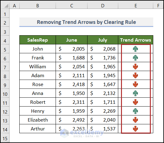
To remove the arrows:
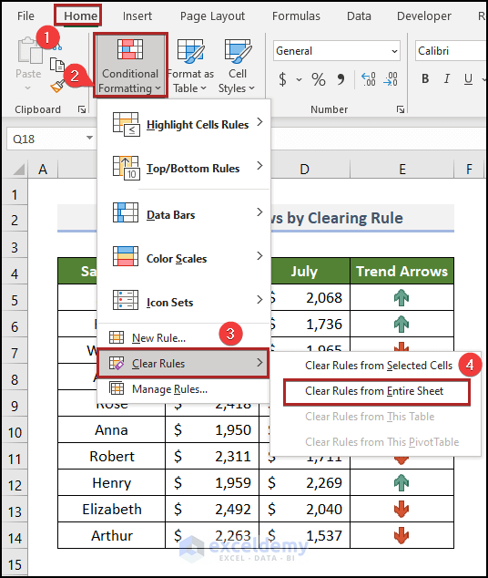
Steps:
- Go to the Home tab.
- Click Conditional Formatting in Styles.
- Select Clear Rules.
- Choose Clear Rules from Entire Sheet.
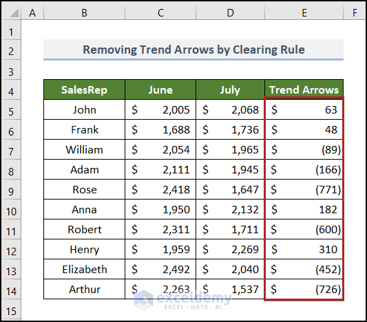
This is the output.
2. Using the Custom Format Option
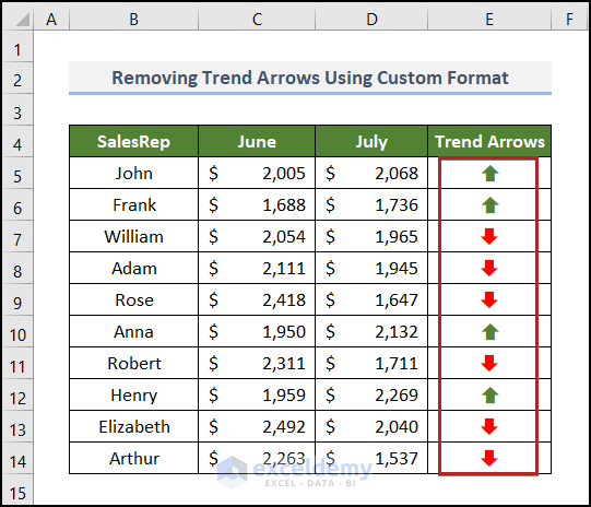 Steps:
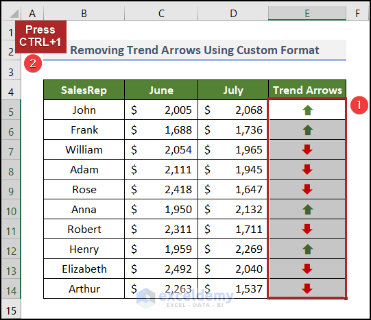
- Select all the trend arrows in E5:E14.
- Press CTRL + 1.
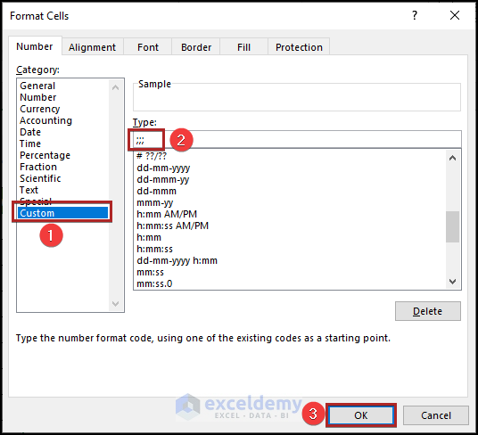
- In the Format Cells dialog box, select Custom in Category.
- In Type, use the code below.
;;;
- Click OK.
This is the output.
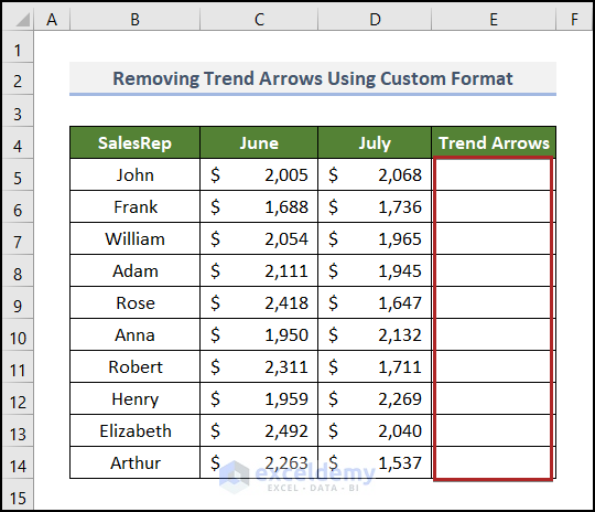
They are still present:
- Select E5 and observe the Formula Bar.
Read More: How to Remove Tracer Arrows in Excel
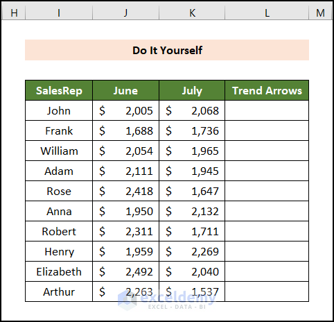
Practice Section
Practice here.
Download Practice Workbook
Download the following Excel workbook.
Related Articles
- How to Insert Curved Arrow in Excel
- How to Use Blue Line with Arrows in Excel
- How to Show Tracer Arrows in Excel
<< Go Back to Arrows in Excel | Excel Symbols | Learn Excel
Get FREE Advanced Excel Exercises with Solutions!
