How to Add Up and Down Arrows in Excel (4 Easy Ways)

You might want to add up and down arrows in Excel so that you can easily understand the increase and decrease in the price of your business commodities and stock price. We can easily make a decision from the up and down arrows from the price of the business commodities and stock. Adding up and down arrows is an easy task. In this article, we’ll learn 4 quick and suitable ways to add up and down arrows in Excel.

How to Add Up and Down Arrows in Excel: 4 Suitable Ways

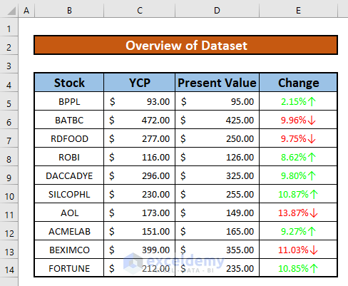
Let’s say, we have a dataset that contains information about several stock companies. The Name of the Stock companies, yesterday’s closing price(YCP), Present Price, and the percentage of change are given in Columns B, C, D, and E respectively. We might add up and down arrows in Excel using the Conditional Formatting, IF Function, Custom Command, and Font Command. Here’s an overview of the dataset for today’s task.

1. Use Conditional Formatting to Add Up and Down Arrows in Excel

In this section, we will apply Conditional Formatting to add up and down arrows in Excel. From our dataset, we can easily add up and down arrows. Let’s follow the instructions below to add up and down arrows!

Steps:

• First, select cell E5. After that, from your Home ribbon, go to,

Home → Styles → Conditional Formatting → Icon Sets → Directional( Select any Set)

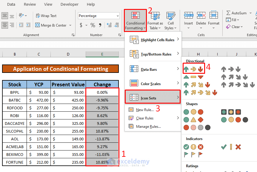
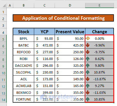
• As a result, you will be able to add up and down arrows which have been given in the below screenshot.

Read More: Up and Down Arrows in Excel Using Conditional Formatting

2. Apply IF Function to Add Up and Down Arrows in Excel

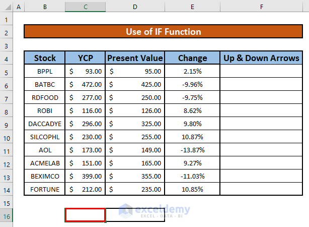
Now, we will apply the IF function to add up and down arrows in Excel. To do that, firstly, you insert up and down arrows from the Symbol option. Let’s follow the instructions below to add up and down arrows using the IF function.

Step 1:

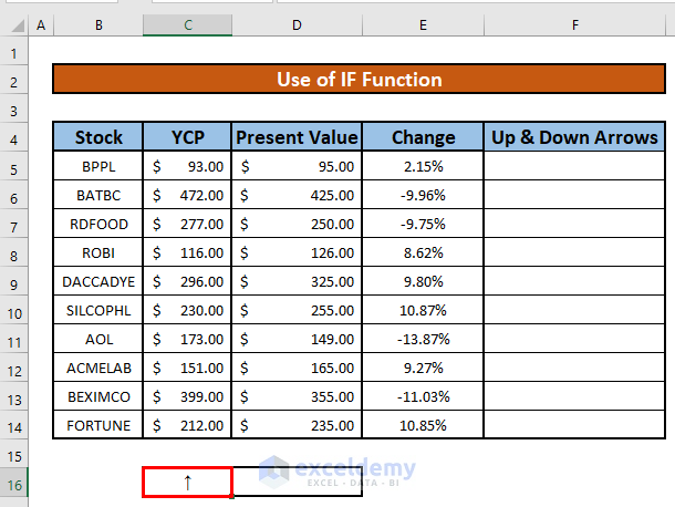
• First, select cell C16.

• Hence, from your Insert ribbon, go to,

Insert → Symbols → Symbol

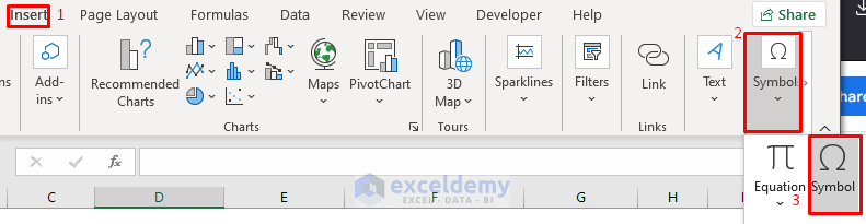
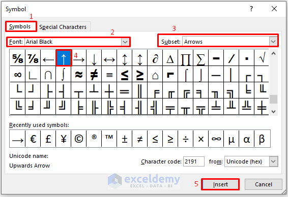
• As a result, a Symbol dialog box will appear in front of you. From the Symbol dialog box, firstly, select the Symbols Secondly, select Arial Black from the Font drop-down list.
• Further, select Arrows from the Subset drop-down list.
• At last, press Insert.

• After that, you will be able to insert the up arrows.

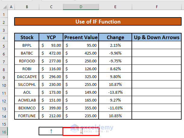
• Similarly, insert the down arrow.

Step 2:

• Now, select cell F5, and write down the IF function in that cell. The IF function is,

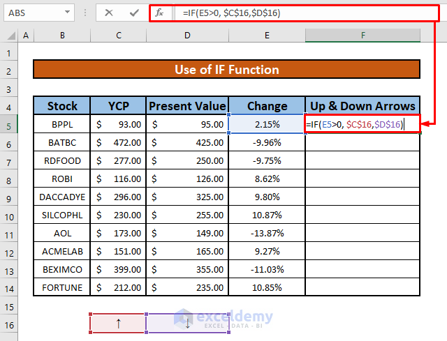
• Hence, press Enter on your keyboard.
• As a result, you will be able to get the return of the IF function.
• The return is up arrow(↑).

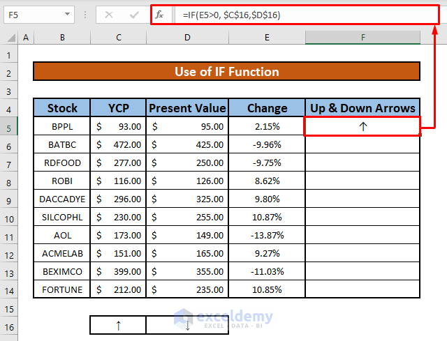
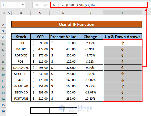
• Further, AutoFill the IF function to the rest of the cells in column F which has been given in the screenshot.

Read More: Double Headed Arrow in Excel

3. Perform Custom Command to Add Up and Down Arrows in Excel

Further, we will perform the Custom Command to add up and down arrows in Excel. We can easily do that from our dataset. Let’s follow the instructions below to add up and down arrows!

Steps:

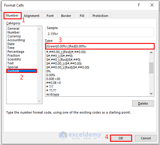
• First, select cells E5 to Hence, press Ctrl + 1 on your keyboard.

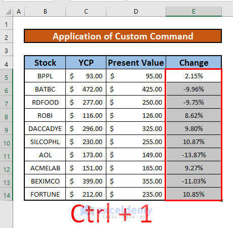
• As a result, a Format Cells dialog box will appear in front of you. From the Format Cells dialog box, firstly, select the Number Secondly, select Custom from the Category drop-down list.
• Further, type [Green]0.00%↑;[Red]0.00%↓ in the Type box.
• At last, press OK.

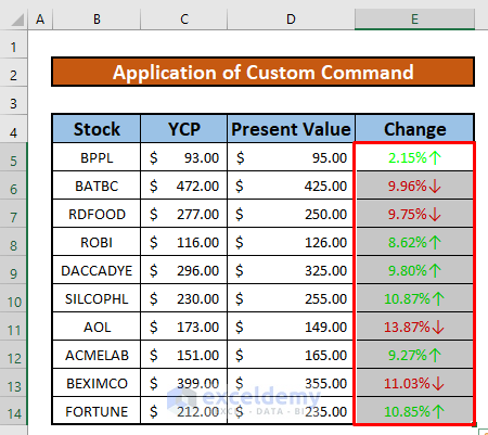
• After completing the above process, you will be able to add up and down arrows which have been given in the below screenshot.

Read More: How to Add Trend Arrows in Excel

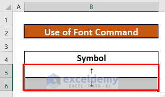
4. Change Font Style to Add Up and Down Arrows in Excel

Last but not least, we will add up and down arrows changing the Font. From our dataset, we can easily do that. This is a time-saving task also. Let’s follow the instructions below to add up and down arrows!

Steps:

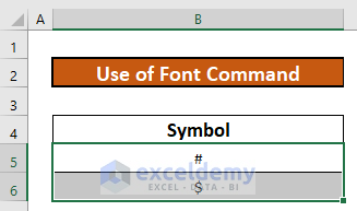
• First, select cells B5 and B6 which contain the Hash(#) and Dollar($) sign.

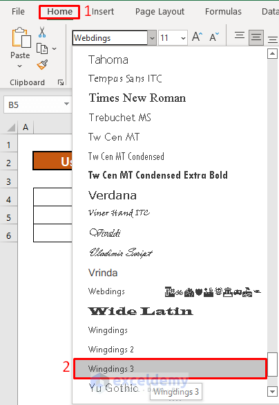
• After that, from your Home ribbon, go to,

Home → Font

• Hence, select Wingdings 3 to convert the Hash(#) and Dollar($) sign into up and down arrows respectively.

• Finally, you will get the up and down arrows that have been given in the below screenshot.

Things to Remember

👉 #N/A! error arises when the formula or a function in the formula fails to find the referenced data.

👉 #DIV/0! error happens when a value is divided by zero(0) or the cell reference is blank.

Download Practice Workbook

Download this practice workbook to exercise while you are reading this article.

Conclusion

I hope all of the suitable steps mentioned above to add up and down arrows will now provoke you to apply them in your Excel spreadsheets with more productivity. You are most welcome to feel free to comment if you have any questions or queries.

Related Articles

• How to Insert Trend Arrows Based on Another Cell in Excel
• How to Show Tracer Arrows in Excel
• How to Remove Tracer Arrows in Excel
• How to Insert Curved Arrow in Excel
• How to Insert Red Arrow in Excel Cell
• How to Use Blue Line with Arrows in Excel

<< Go Back to Arrows in Excel | Excel Symbols | Learn Excel