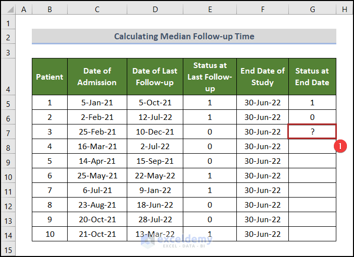
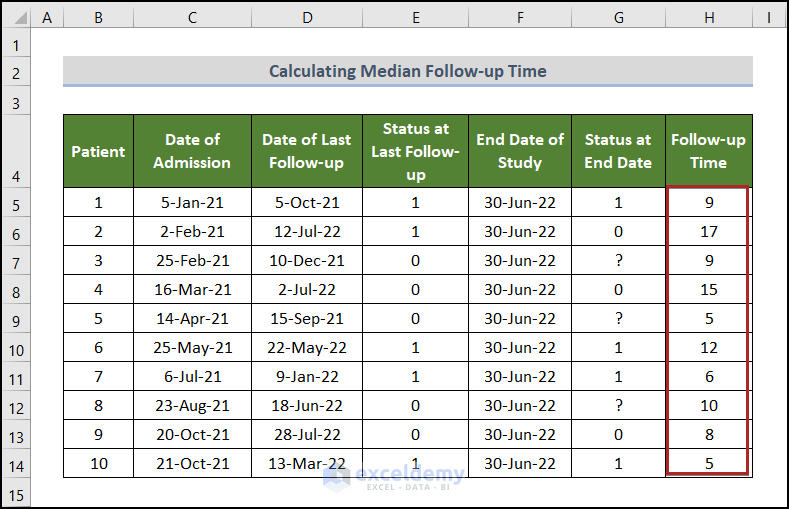
The dataset showcases a Follow-up History of 10 Cancer Patients.
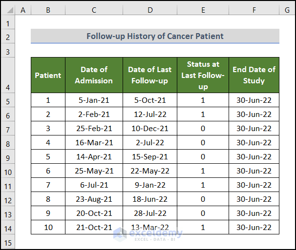
1 and 0 indicate the status of the patient at the time of the last follow-up. 1 means dead and 0 means still alive.
Calculate the median follow-up time of this study:
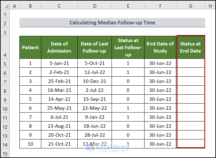
Step 1 – Determine the Status at the End Date
Steps:
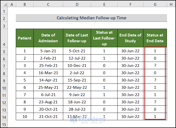
- Create a new column: Status at End Date.
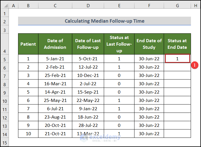
To enter the end status of patient 1 in G5:
Mind the data for Patient 1 in Row 5. His admission was on 5 Jan 2021 and his last follow-up was on 5 Oct 2021. On that date, he was already dead (1 in E5). By the end of this study, on June 30, 2022, his status is dead: the end date is after the last follow-up.
- Go to G5 and enter 1.
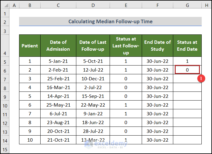
As for the second patient:
His admission date was on 2 Feb 2021 and the last follow-up on 12 Jul 2022, which is beyond the end date of the study. At that time, he was dead. At the end date of the study, he was alive. He died on 12 Jul 2022.
- Select G6 and enter 0.
The third patient’s admission date was on 25 Feb 2021 and his last follow-up was on 10 Dec 2021. At that time, he was alive. The status of the end date is uncertain.
- In G7, enter a ?.
- Enter data in G8:G14.
Read More: How to Calculate Percentage of Time in Excel
Step 2 – Calculate the Follow-up Time of Each Patient
Steps:
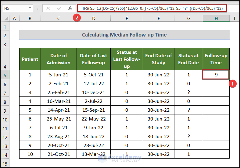
- Select H5 and enter the following formula.
=IFS(G5=1,((D5-C5)/365)*12,G5=0,((F5-C5)/365)*12,G5="?",((D5-C5)/365)*12)
The IFS function returns a value if the first condition is met.
There are 3 conditions and 3 outputs:
- In the first condition, if the value in G5 equals 1, the formula will return the value of ((D5-C5)/365)*12 in H5. It is divided by 365 to get it in years and then multiplied by 12 to get the final output in months.
- Output → ((44474-44201)/365)*12 → 8.97 (in H5, 9 as there are no decimals)
- G6 displays 0. The return value is ((F6-C6)/365)*12 in H6.
- Output → 17
- Press ENTER.
- Double-click the Fill Handle tool.
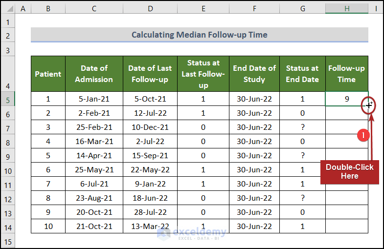
The formula is copied to the rest cells in the Follow-up Time column.
Step 3 – Find out the Median Follow-up Time
Steps:
- Go to H15 and use the following formula.
=MEDIAN(H5:H14)
The MEDIAN function returns the median of a group of numbers in H5:H14.
- Press ENTER.
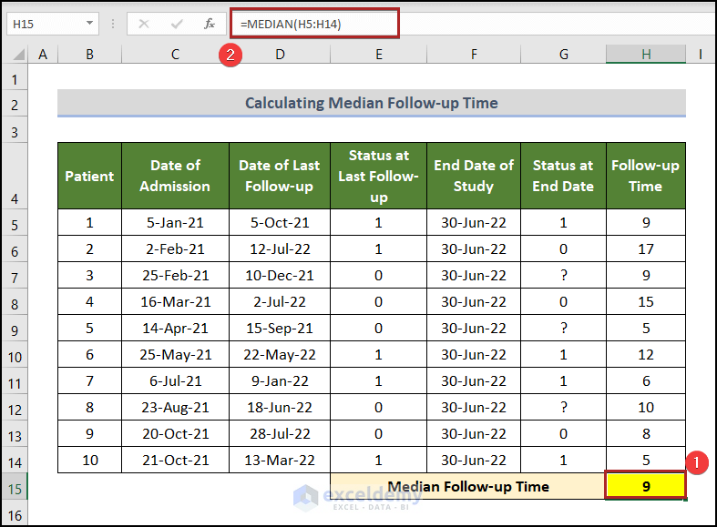
This is the output.
Read More: How to Calculate Lead Time in Excel
Median Follow-up vs Median Survival
Median follow-up and median survival time are commonly used terms in the medical sector.
The median survival time is a time point in the research period, indicating that 50% of the patients are alive. In the survival analysis graph, the median survival time is the point where the S(t) function meets 0.50 on the survival curve, .
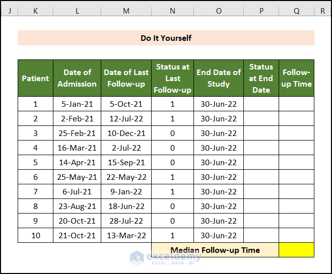
Practice Section
Practice here.
Download Practice Workbook
Download the following Excel workbook.
Related Articles
- How to Calculate Total Hours in Excel
- How to Calculate Total Time in Excel
- How to Calculate the Duration of Time in Excel
- How to Calculate Lag Time in Excel
- How to Sum Time in Excel
- [Fixed!] SUM Not Working with Time Values in Excel
<< Go Back to Calculate Time | Date-Time in Excel | Learn Excel
Get FREE Advanced Excel Exercises with Solutions!

Bonjour,
Really enjoyed reading your article. Here you enter the end status manually, but i understand that it could be done with formula, but can’t figure out how. show me some light on this.please.thank you very much.
Hello Elaine,
First, it feels good to see your interest in learning it. That motivates us to work hard.
Now, coming back to your question. Here you intend to enter the End Date Status automatically. Yes, that’s a very good thought. In this era of automation, why should we lag behind? Hahahaha…. Okay, let’s get to the solution now.
There could be 4 separate conditions. First, the Last Follow-up Date could be before the End Date of the study and the patient is dead at the Last Follow-up Date. Second, the Last Follow-up Date could be after the End Date of the study and the patient is dead at the Last Follow-up Date. Third, the Last Follow-up Date could be before the End Date of the study and the patient is alive at the Last Follow-up Date. And the fourth, the Last Follow-up Date could be after the End Date of the study and the patient is alive at the Last Follow-up Date. So, how can we determine the End Date Status for these situations? Let’s see the steps below.
• Firstly, go to cell G5 and enter the following formula.
=IFS(AND(E5=1,D5<F5),1,AND(E5=1,D5>F5),0,AND(E5=0,D5<F5),"?",AND(E5=0,D5>F5),0)Here, we used the IFS function where we inserted those 4 conditions as logical_test and their output as value_if_true. Further, we used the AND function to join two conditions together.
• Finally, press ENTER.
That’s all from me on this. Don’t forget to visit our website, Exceldemy, a one-stop Excel solution provider, to explore more.
Stay well and healthy. Happy Excelling ☕.