How to Calculate Lag Time in Excel (2 Methods)

What Is Lag Time?

Lag Time or Time Lag is a delay between two successive tasks, whereas the later task should start as soon as the earlier task ends. Suppose a project consists of 5 successive tasks. Each task should start as soon as the previous task ends. But each new task started after a delay due to mechanical failures and other difficulties. Then this delay itself is the time lag. You can sum up all the delays to get the total time lag. It will be equal to the difference between the projected deadline and the actual deadline of the project.

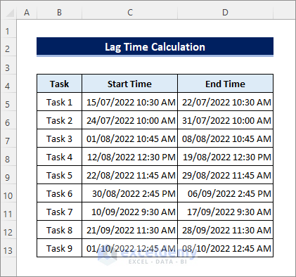
Method 1 – Calculate the Lag Time Between Consecutive Tasks

Scenario: Suppose you have a dataset with the start and end times of tasks within a project. There’s a delay between the start of each task and the end of the previous task.

Objective: Calculate the lag time between consecutive tasks.

Formula:

• In cell E6, enter the following formula:

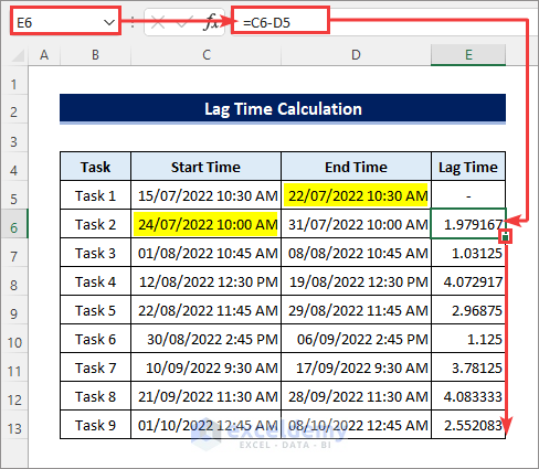
Here, C6 represents the start time of task 2, and D5 represents the end time of task 1.

• Drag the Fill Handle icon down to apply the formula to the entire range (E6:E13).

Formatting:

• Select the range E6:E13.
• Go to Home > Format > Format Cells (or use the CTRL+1 shortcut).
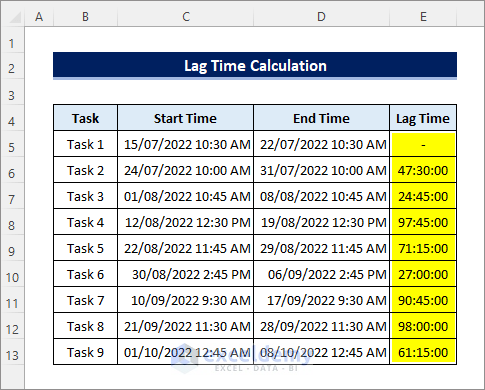
• Choose the “37:30:55” format in the Time category from the Number tab and click OK.

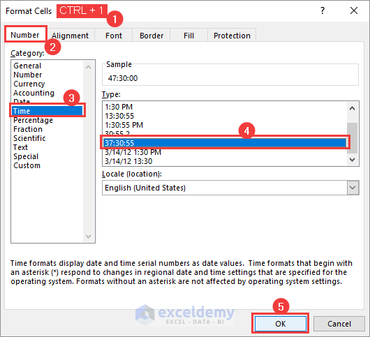
• You’ll now have the lag time between tasks.

Read More: How to Calculate Lead Time in Excel

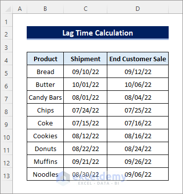
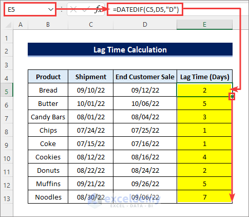
Method 2 – Calculate the Lag Time Between Shipment and End-Customer Sale

Scenario: Suppose you want to calculate the time lag between shipment and end-customer sales for your company’s products.

Formula:

• In cell E5, enter the DATEDIF function:

• • • This will give you the lag time in days.
• Drag the Fill Handle icon down.

Things to Remember

• Always subtract the earlier date from the later date to avoid negative results.
• The DATEDIF function isn’t explicitly listed in Excel, but you can still use it (with some limitations).

Download Practice Workbook

You can download the practice workbook from here:

Related Articles

• How to Calculate Median Follow-up Time in Excel
• How to Calculate Total Hours in Excel
• How to Calculate Total Time in Excel
• How to Calculate the Duration of Time in Excel
• How to Calculate Percentage of Time in Excel
• How to Sum Time in Excel
• [Fixed!] SUM Not Working with Time Values in Excel

<< Go Back to Calculate Time | Date-Time in Excel | Learn Excel