Introduction to Holt-Winters Exponential Smoothing
The Holt-Winters method is an advanced method to forecast values. It considers seasonality, and trend effects while predicting the forecast.
The formula is:
Ft+k = (Lt+k*Tt)*St-m+k
Where, F = Forecasted Value
L = Level
T = Trend
M = 4 for the quarterly period, 12 for the monthly period
S = Seasonality Index
This is the sample dataset.
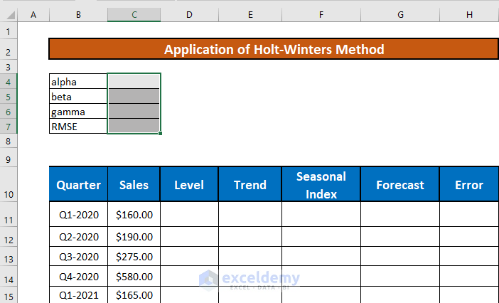
you want to calculate the forecast values for 2023.
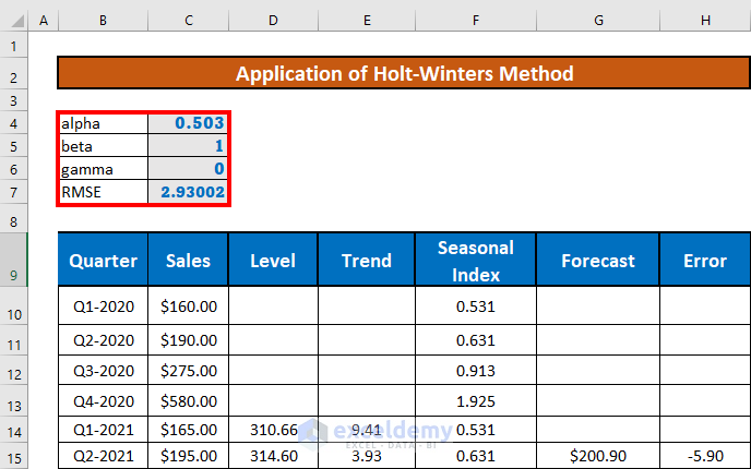
Step 1 – Assign Random Alpha, Beta & Gamma Values
- Assign random values to the constants alpha, beta, and gamma.

These values will be later optimized.
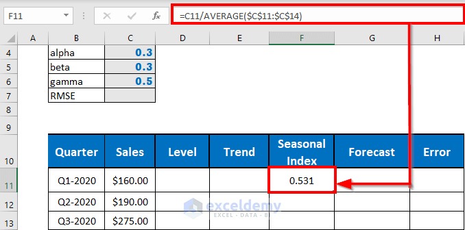
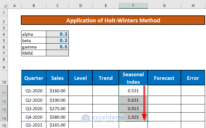
Step 2 – Calculate the Initial Seasonal Index
- Go to F11 and enter the following formula.
=C11/AVERAGE($C$11:$C$14)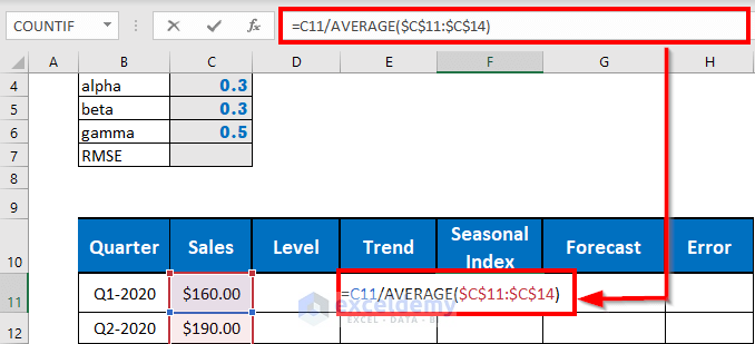
- Press ENTER.
- This is the output.
- Drag down the Fill Handle to F14.
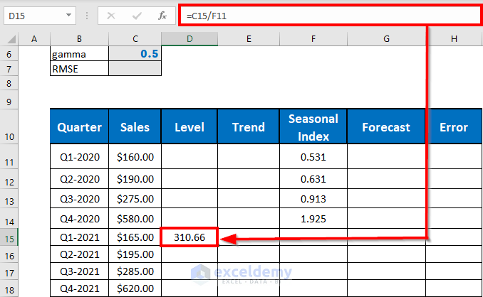
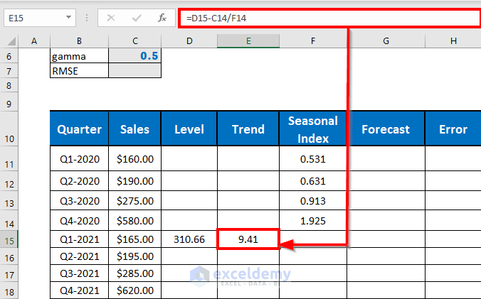
Step 3 – Determine the Initial Level and Trend
The initial level is the level of the 5th quarter .
The formula is:
L5 = Y5/S1
Y5= Sales of the 5th Quarter.
S1= Seasonal Index of the 1st Quarter.
- Go to D15 and enter the formula:
=C15/F11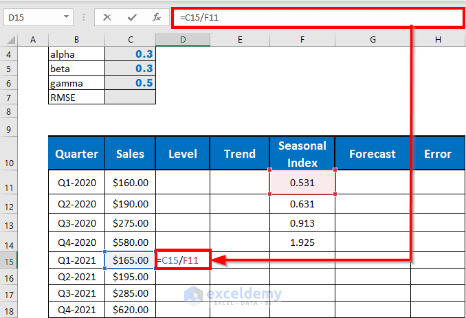
- Press ENTER.
This is the output.
Calculate the initial trend:
T5 = L5-Y4/S4
Where, L5 = Level for 5th Quarter.
Y4 = Sales for the 4th Quarter.
S4 = Seasonal Index for 4th Quarter.
- Go to E15 and enter the formula,
=D15-C14/F14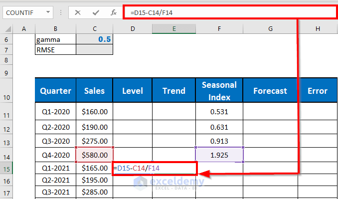
- Press ENTER.
This is the output.
Step 4 – Calculate the Next Seasonal Indexes
The general formula to calculate the seasonal index is:
St = ɣ(Yt/Lt)+(1-ɣ)St-m
L = Level.
T = Trend.
M = 4 for the quarterly period, and 12 for the monthly period.
S = Seasonality Index.
Ɣ = Coefficient.
- Go to F15 and enter the following formula
=$C$6*(C15/D15)+(1-$C$6)*F11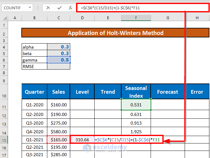
- Press ENTER.
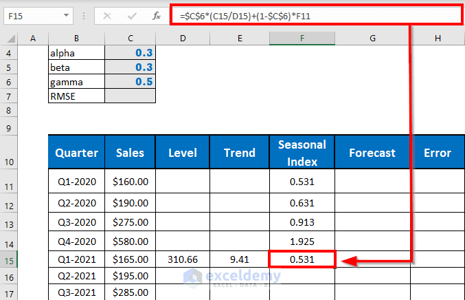
- Drag down the Fill Handle to see the result in the rest of the cells.
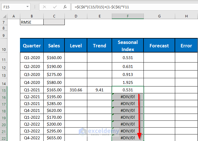
Note: Ignore the error (it will disappear once you measure the next Levels and next Trends).
Step 5 – Determine the Next Levels
This is the formula.
Lt = α(Yt/St-m)+(1-α)(Lt-1+Tt-1)
L = Level
T = Trend
M = 4 for the quarterly period, 12 for a monthly period
S = Seasonality Index
α = Coefficient
- Go to D16 and enter the following formula.
=$C$4*(C16/F12)+(1-$C$4)*(D15+E15)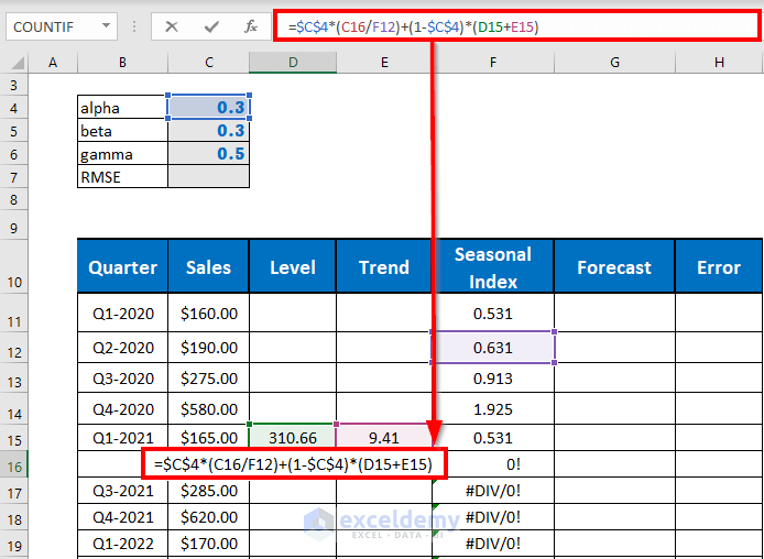
- Press ENTER.
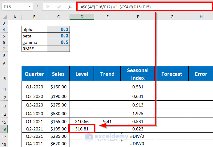
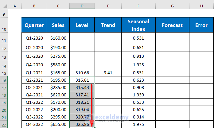
- Drag down the Fill Handle to see the result in the rest of the cells.
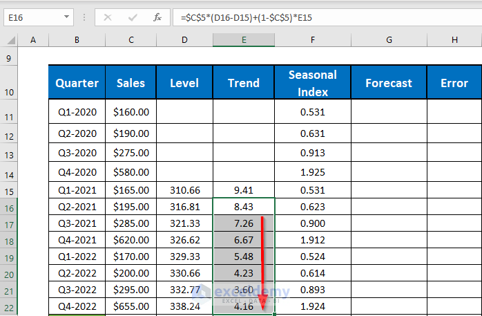
Step 6 – Measure the Next Trends
The formula is:
Tt= β(Lt-Lt-1)+(1-β)Tt-1
L = Level
T = Trend
M = 4 for the quarterly period, 12 for a monthly period
S = Seasonality Index
β= Coefficient
To calculate the trend effect:
- Go to E6 and enter the following formula
=$C$5*(D16-D15)+(1-$C$5)*E15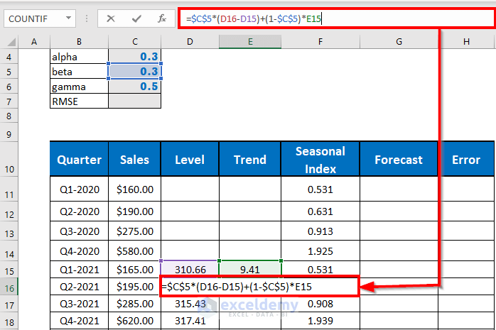
- Press ENTER.
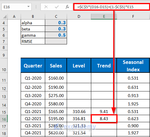
- Drag down the Fill Handle to see the result in the rest of the cells..
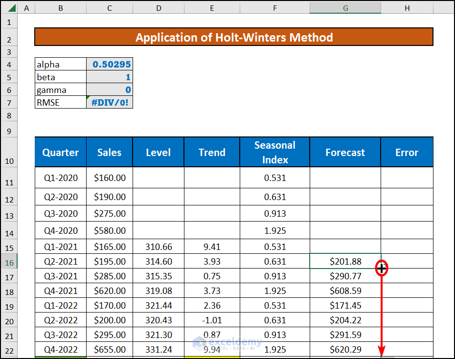
Step 7 – Find the Forecast Values to Compare with Actual Sales
The formula to calculate the forecast values (for comparison) is:
Ft = (Lt-1 + Tt-1)* St-M
- Go to G16 and enter the following formula
=(D16+E16)*F12
- Press ENTER.
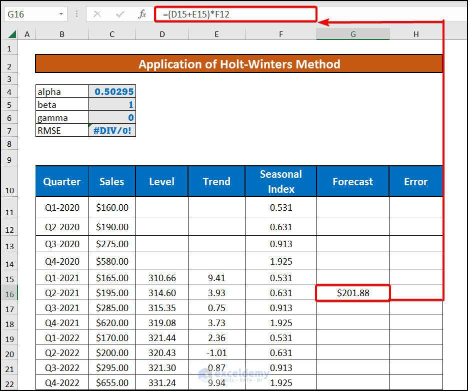
- Drag down the Fill Handle to see the result in the rest of the cells.
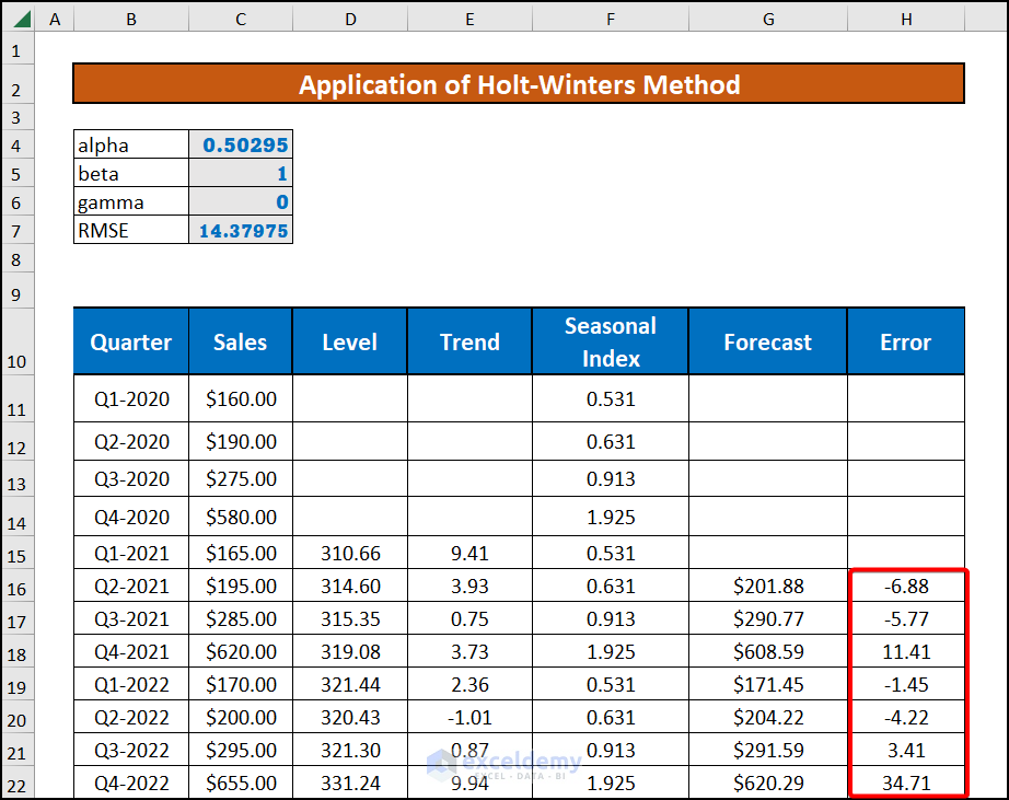
Step 8 – Calculate Forecasting Errors
- Go to H16 and enter the formula.
=C16-G16
- Press ENTER.
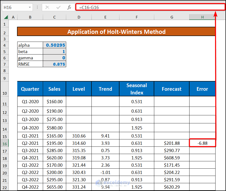
- Drag down the Fill Handle to see the result in the rest of the cells.
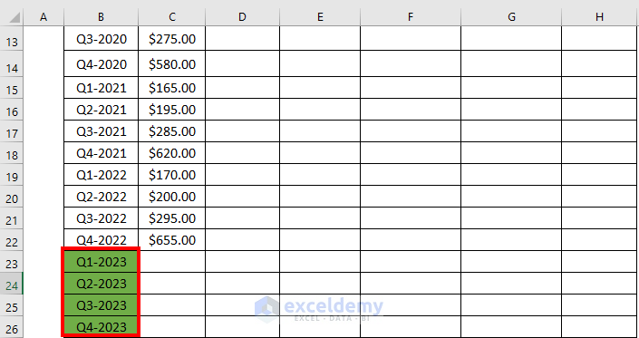
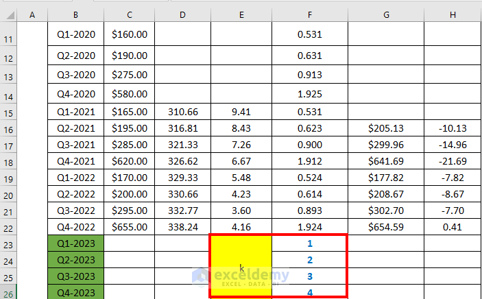
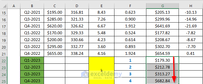
Step 9 – Assign a K Value to Quarters to Be Forecast
The co-efficient k represents the future time to forecast. Calculate the forecast for the 4 quarters of 2023 based on the 2022 available data.
Step 10 – Calculate the Forecast Value
Use the last available Level, Trend, and Seasonality to calculate it.
- Go to G23 and enter the following formula.
=($D$22+F23*$E$22)*F19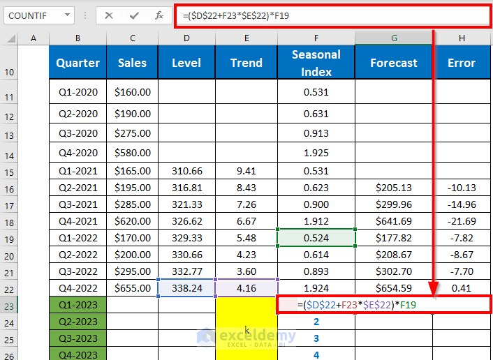
- Press ENTER to see the output.
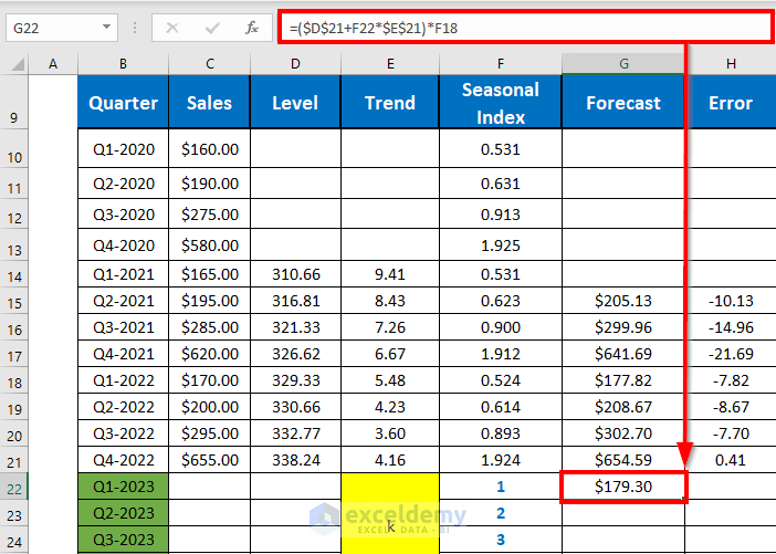
- Drag down the Fill Handle to see the result in the rest of the cells.
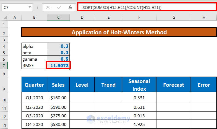
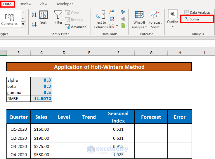
Step 11 – Optimize Alpha, Beta, and Gamma
To minimize errors, optimize the values of alpha, beta, and gamma, using the Excel solver.
- Calculate the root mean square error: go to C7 and enter the following formula.
=SQRT(SUMSQ(H15:H21)/COUNT(H15:H21))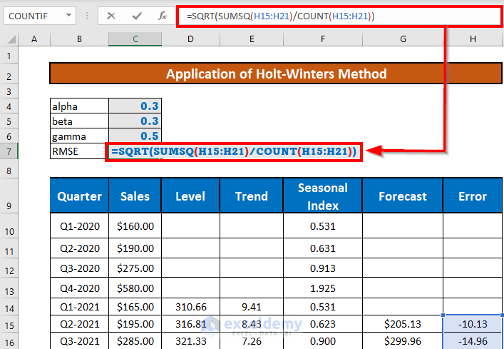
Formula Breakdown:
- COUNT(H15:H21) → Counts the number of cells.
- Output → 7
- SUMSQ(H15:H21) → Calculatesthe sum of the squares of H5:H11.
- Output → 463493653301
- =SQRT(SUMSQ(H15:H21)/COUNT(H15:H21)) → Calculates the RMSE
- =SQRT(992.463493653301/7)
- =SQRT(141.780499093329)
- Output → 9072
- Press ENTER.
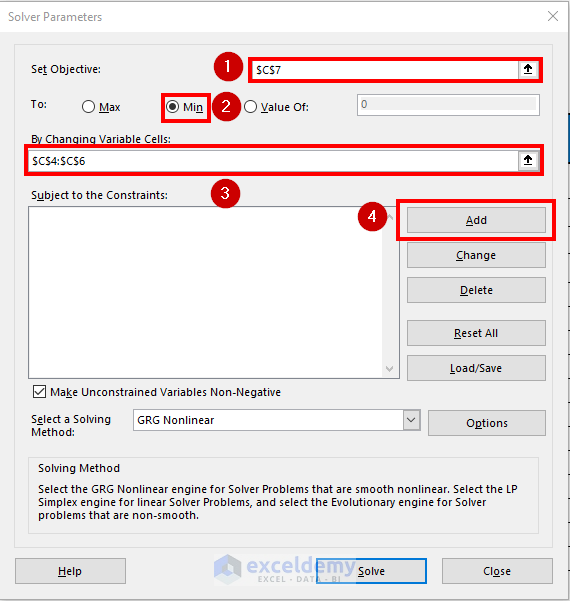
- Go to the Data tab >> select Solver.
- In the Solver Parameters window, set RMSE to minimum by changing the values of the coefficients.
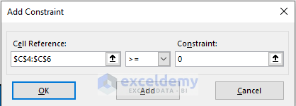
- To add constraints, click Add.
- In the Add Constraint window, set the cell reference and value. The constraints are 0<=α,४,ß<=1
- Add the second constraint. Click Solve.
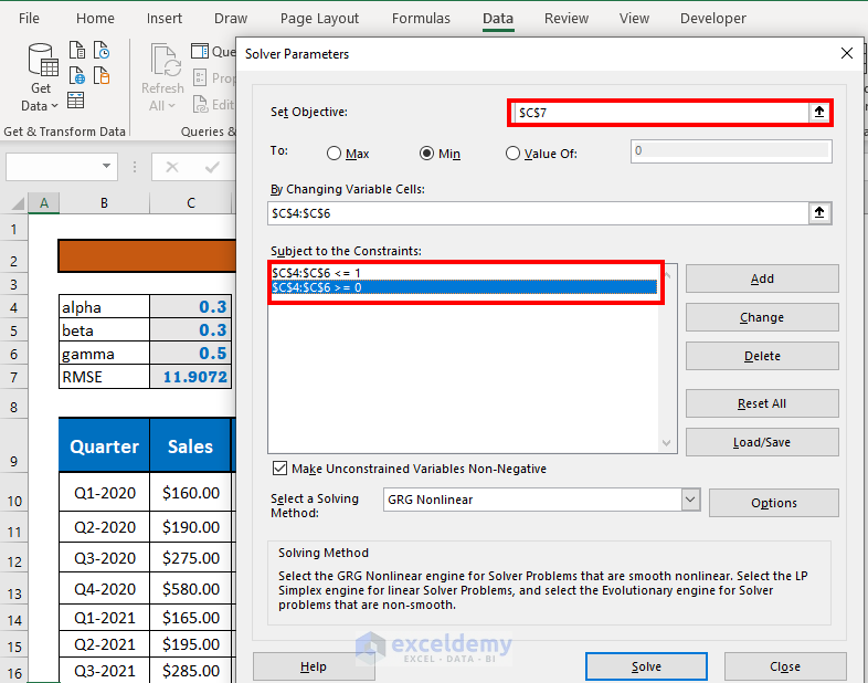
- Excel will minimize the error by optimizing alpha, beta, and gamma.
Things to Remember
- Activate the solver add-in.
Download Workbook
Download the workbook and practice.
Related Articles
- How to Calculate Trend Adjusted Exponential Smoothing in Excel
- How to Remove Noise from Data in Excel
- How to Smooth Data in Excel
<< Go Back to Exponential Smoothing in Excel | Solver in Excel | Learn Excel
Get FREE Advanced Excel Exercises with Solutions!

Thanks for Holt’s Winter excel spreadsheet. It helped a Lot. Are there more examples. I enjoyed the one you sent.
Thank you for your kind words.
Have a good day!!
Hola! Estoy intentando usar el pronóstico para kilogramos de un artículo en doce meses, pero no logro que la cantidad de kilogramos del año 2023 tenga sentido. El año 2022 son 3000 kg y el año 2023 1200, algo tengo mal… Por favor, ¿podría pasarme un ejemplo del excel para 12 meses? Gracias!
English: Hello! I’m trying to use the forecast for kilograms of an item in twelve months, but I can’t get the number of kilograms for the year 2023 to make sense. The year 2022 is 3000 kg and the year 2023 is 1200, I have something wrong… Please, could you give me an example of excel for 12 months? Thank you!
Hi JORGE,
It’s a bit difficult to answer this, not seeing your spreadsheet. Can you please send a sample to [email protected]?
Prior to that, check the following Excel file. We have added a 12-month example for you. Let us know if this helps.
Download Link:
Solution.xlsx
Note:
You must have data of 2021 and 2022 for forecasting 2023.
hi dear
hope you are fine
as i checked your spread sheet , it need to years data , i have data for 14 month , i have tried to use it , but not performed , plz help me
abolfazl
Hello Abolfazl,
Hope you’re doing well. Since Holt-Winters Exponential Smoothing requires a proper trend and seasonality pattern, having 14 months of data might not be enough for accurate forecasting, depending on your dataset’s characteristics.
Could you check if your data includes a clear seasonal pattern? Also, ensure that your time series data is structured correctly in Excel, following the smoothing model requirements.
Since Holt-Winters Exponential Smoothing requires at least two years of data to capture seasonality properly, having only 14 months may not provide an accurate forecast. However, you can try the following steps to improve your model:
Solution:
Extend Data Period: If possible, include more historical data (preferably at least 24 months) to allow Excel to detect trends and seasonal variations better.
Use Moving Averages Instead:
1. If you don’t have a full two years of data, try a Simple Moving Average (SMA) or Exponential Smoothing (without seasonality) to get a trend-based forecast.
2. In Excel, use =AVERAGE(range) for a moving average.
Apply Holt’s Linear Trend Model (if seasonality is not strong):
1. Instead of the triple exponential smoothing, use Holt’s method (Double Exponential Smoothing) in Excel.
2. Go to Data → Forecast Sheet and select Linear Forecast instead of Seasonal.
Check Alpha, Beta, and Gamma Parameters:
1. If you are using Holt-Winters in Excel, ensure that Alpha (Level), Beta (Trend), and Gamma (Seasonality) values are properly adjusted.
2. Try reducing Gamma or setting it to zero if seasonality is not evident.
If your dataset has irregular patterns, a linear regression model in Excel using LINEST or FORECAST.ETS.LINEAR might work better for short-term predictions.
Let me know if you need further details!
Best regards,
ExcelDemy
Hi Akib,
I think G16 should be: =(D15+E15)*F12 instead of =(D16+E16)*F12, right?
Thank you.
Hi Quang,
Thanks for your feedback. You are right on this occasion. The formula will be
=(D15+E15)*F12in G16. unfortunately, we have made a mistake here. Thanks to you that you corrected us. We have updated the article.Best wishes to you.
Regards
Fahim Shahriyar Dipto
Excel & Content Developer.