How to Create a 50-30-20 Budget Spreadsheet in Excel

Step 1 – Calculate Monthly Income

For illustration, we have a sample Monthly Income dataset with a column for sources of income in the B5:B8 range. The income sources are salary, overtime pay, additional income, and others.

Insert a new column for the amount under Column C.

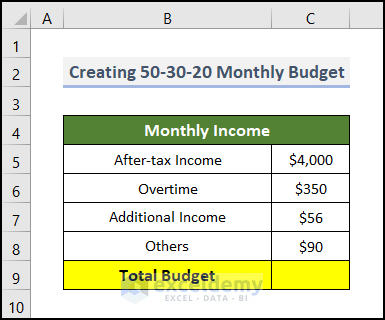
Calculate the Total Budget from the incomes.
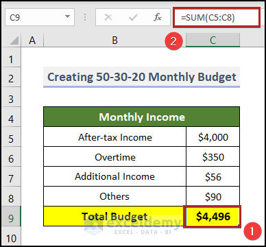
To do this, select cell C9 and enter the following formula.

=SUM(C5:C8)

C5:C8 represents the range of amounts for several types of income sources.

Press ENTER.

Step 2 – Determine Ideal 50-30-20 Division

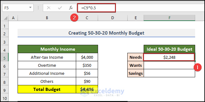
Go to cell F5 and add the following formula in the Formula Bar.

=C9*0.5

Since the Needs is 50% of the total income, we multiplied the Total Budget in cell C9 by 0.5.

Press the ENTER key.

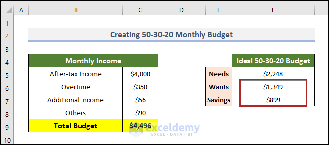
Work out the ideal amount of Wants and Savings.
Take the multiplier as 0.3 to calculate the amount of Wants, and 0.2 for Savings.

Step 3 – Compute Expenses in 3 Different Categories

Calculate the Needs, Wants, and Savings separately.

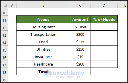
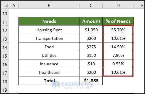
Make a table for Needs expenses.
In Column B, enter the numerous areas of expenses, e.g., Housing Rent, Food, etc.

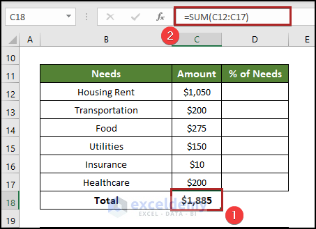
Select cell C18 and add the formula below.

=SUM(C12:C17)

The SUM function will sum up the total expenses for our needs.

Hit ENTER.

To figure out the % of Needs of each Needs category on the list, go to cell D12 and add the following formula.

=C12/$C$18

Press ENTER.

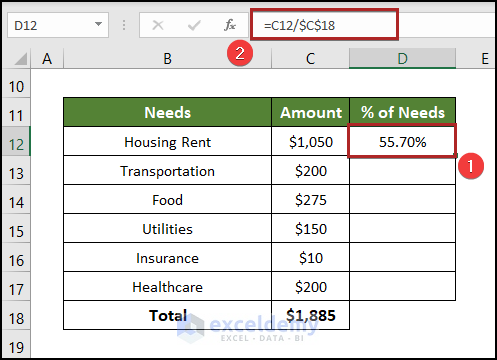
Note: Don’t forget to change the format of cells in D12:D17 to Percentage.

Hover the cursor on the bottom-right corner of cell D12 to get the Fill Handle tool (+). Double-click on it to copy the formula to the rest of the cells in that column.

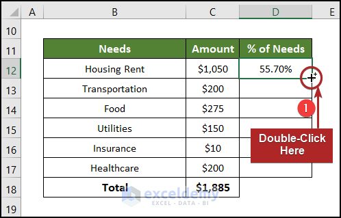
It will give the % of Needs for all categories.

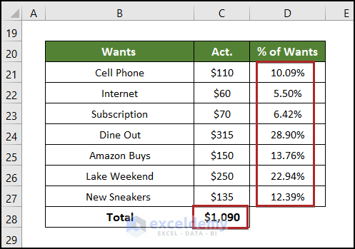
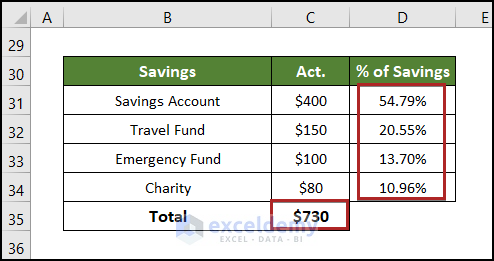
Follow the same procedure for Wants and Savings.

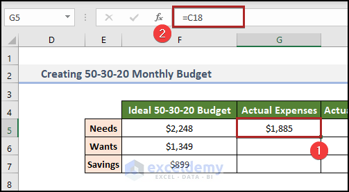
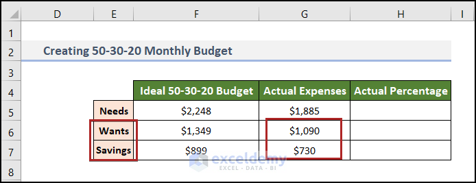
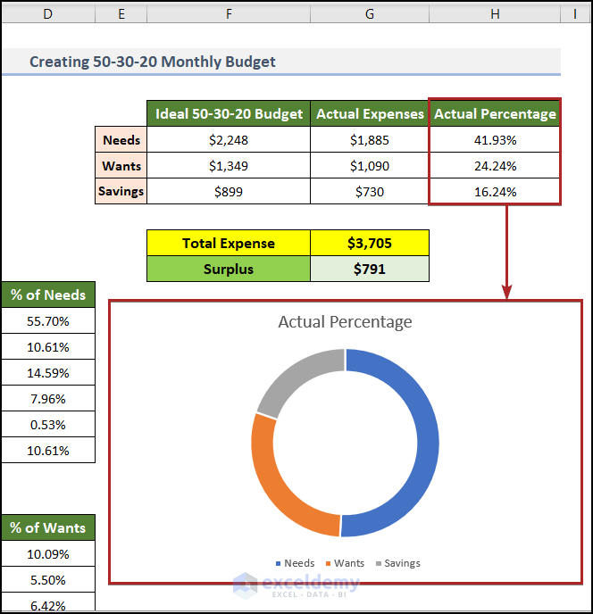
Step 4 – Compare Actual Expenses with the Ideal Budget

Select cell G5 and put in the following formula.

=C18

C18 serves as the cell reference for Total Needs. We’re fetching this value from cell C18 to cell G5.

Press ENTER.

Fetch the values of the Total of Wants and Savings from cells C28 and C35 to cells G6 and G7 respectively.

In Step 2, we calculated an ideal amount of Needs, Wants, and Savings. But, after bearing all expenses for the month, obviously, the percentage of these 3 categories should be different. To test this:

Select cell H5 and add the following formula.

=G5/$C$9

We’re calculating the Actual Percentage of Needs to the Total Budget.

Hit ENTER.

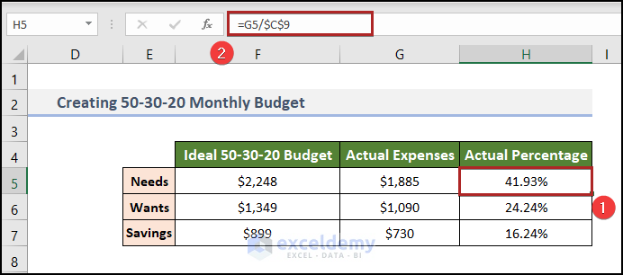
The Actual Percentage of Needs is 41.93%. Whereas we initially allotted it 50%. So, the actual expenditure is less than the ideal amount.

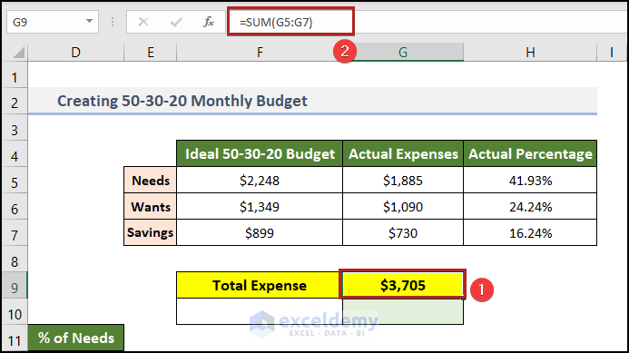
Step 5 – Determine Surplus or Shortage

Select cell G9 and enter the following formula.

=SUM(G5:G7)

We added all the costs here.

Press ENTER.

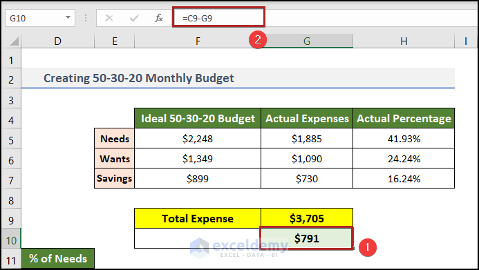
Go to cell G10 and add the formula below.

=C9-G9

We are subtracting the Total Expense from the Total Income.

Hit ENTER.

Go to cell F10 and enter the following formula.

=IF(G10>0,"Surplus","Deficit")

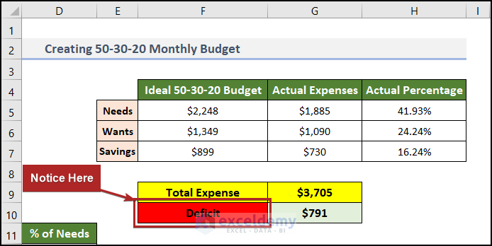
IF function inserts a logical test. If the value in cell G10 becomes greater than 0, then it will show a text string Surplus in cell F10. Otherwise, it will show Deficit in cell F10.

Press ENTER.

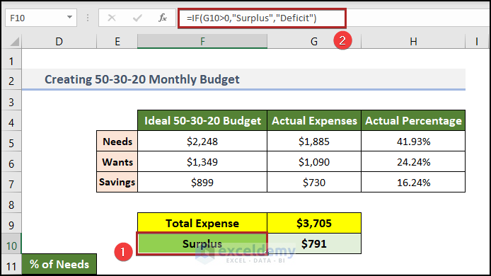
You can also apply Conditional Formatting in cell F10. In the above image, you can see a Green fill color in cell F10. When it is Surplus, it will be Green. And, it will look Red if it is Deficit.

Step 6 – Insert Chart to Visualize Easily

Go to the Insert tab.
Click on the Insert Pie or Doughnut Chart drop-down icon.
Select the Doughnut chart from the available options.

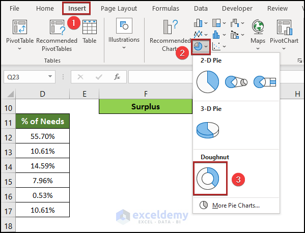
It will add a blank chart on the sheet.

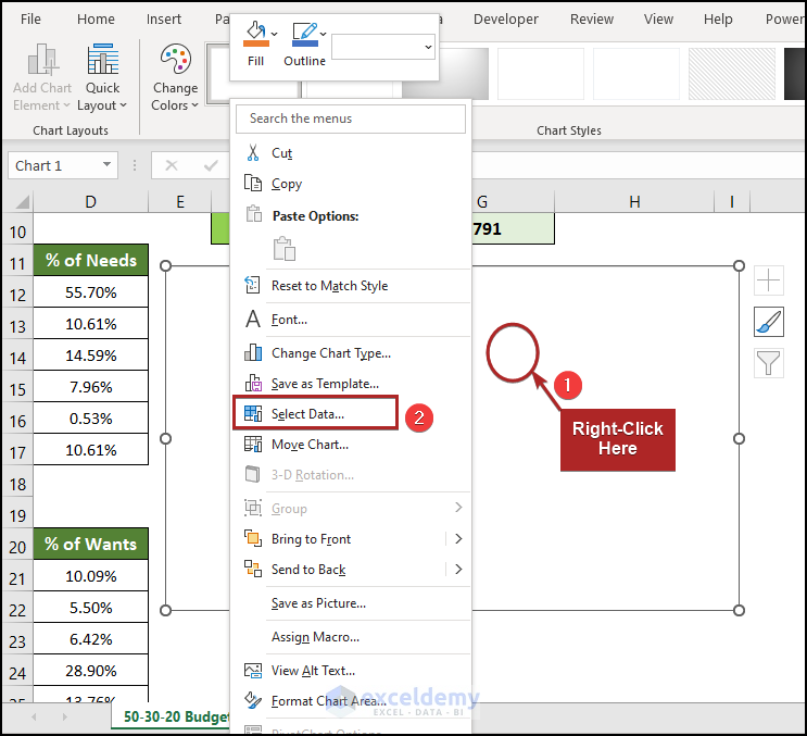
Right-click anywhere on the chart area.

The context menu will pop up.

Choose Select Data from the menu.

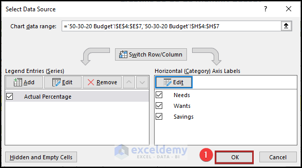
The Select Data Source dialog box will open.

Select the Add button under the Legend Entries (Series) section.

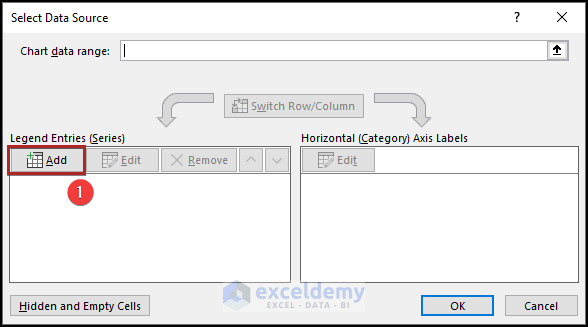
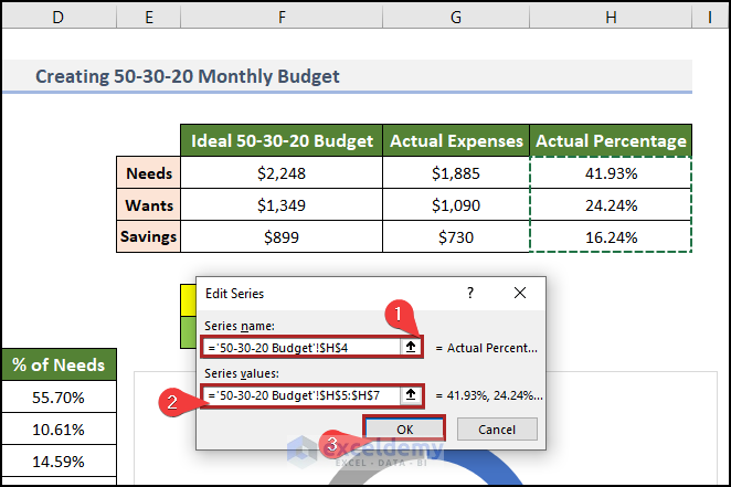
The Edit Series input box will pop up.

In the Series name box, give the reference of cell H4 which is the Actual Percentage.
In the Series values box, give the reference of the H5:H7 range.
Click OK.

Click on the Edit button under the Horizontal (Category) Axis Labels section.

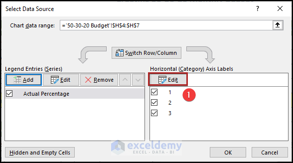
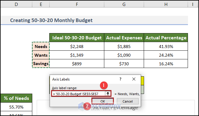
The Axis Labels input box will pop up.

Give the reference of the E5:E7 range in the Axis label range box.
Click OK.

Click OK on the Select Data Source dialog box.

It inserts a chart of the Actual Percentage on the spreadsheet.

Add Data Labels to the chart from the Chart Elements options.

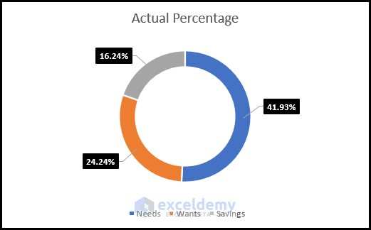
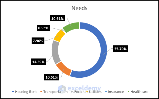
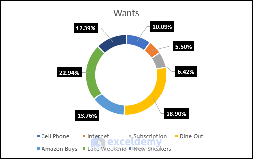
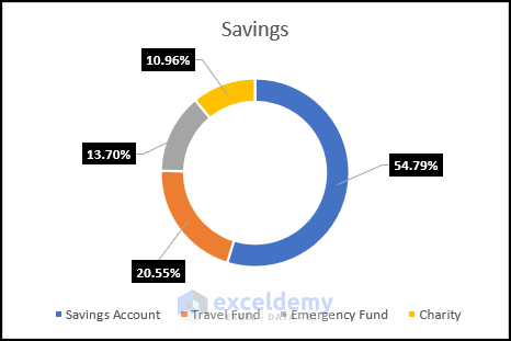
You can introduce charts for various analyses. We’ve added charts for visualizing the percentage of different components of Needs, Wants, and Savings.

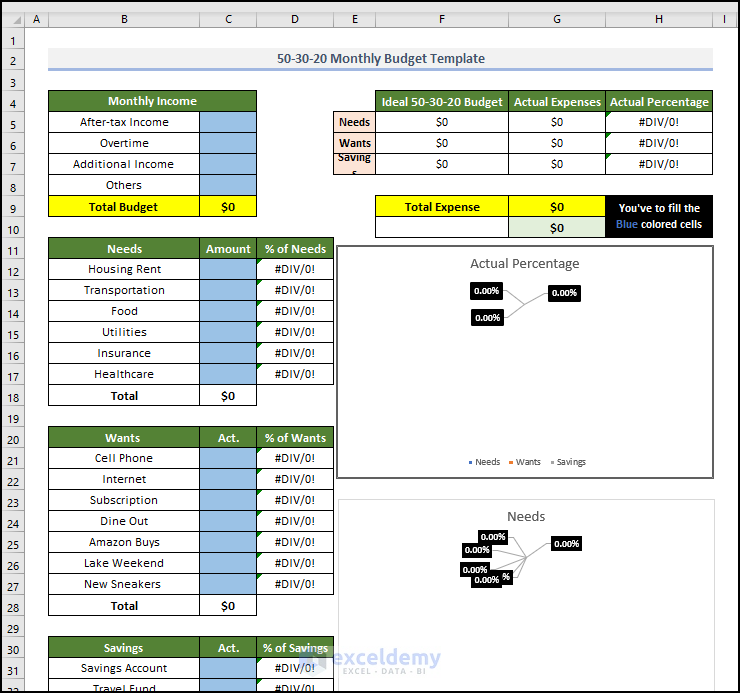
Free Template: Ready to Use

In this workbook, we have added an extra sheet with a free 50-30-20 monthly budget template. You can change and edit it according to your needs. Add your data to the blue-colored cells and calculations will be done automatically.

Download Practice Workbook. Free 50-30-20 Monthly Budget Template Included.

50-30-20 Budget Spreadsheet.xlsx

<< Go Back to Budget Template | Finance Template | Excel Templates

Get FREE Advanced Excel Exercises with Solutions!

2 Comments

Barry Jun 26, 2023 at 1:14 AM

Thank you very much, this is excellent and I have now created this budget. I would like to create this for every month, so can I simply use the Sheet – Move/Copy function to copy this to 12 sheets for every month?
- Reply
  Shahriar Abrar Rafid Jun 26, 2023 at 12:18 PM
  Hi BARYY,
  Thanks for your appreciation. I feel very happy that my tutorial helped you. Now, get back to your query.
  Yes, you can simply Copy the worksheet. Assume, we named the worksheet “Jan” for the month of January.
  Right-click on the sheet name tab and select Move or Copy from the context menu.
  
  In the Move or Copy dialog box, select move to end and check the box of the Create a copy option. Then, click OK.
  
  But, this procedure is lengthy and time-consuming. Because you have to repeat this process 11 times for the remaining 11 months. Also, you have to rename the sheets according to the month’s name. Instead, you can use a simple VBA macro to do it in a click.
  In the Visual Basic Editor, click Insert >> Module.
  
  Paste the following code into the module and click on the Run button.
```
Sub Create_Monthly_Sheets()
Dim monthNames As Variant
Dim i As Integer

monthNames = Array("Feb", "Mar", "Apr", "May", "Jun", "Jul", "Aug", "Sep", "Oct", "Nov", "Dec")

Application.ScreenUpdating = False

' Copy the "Jan" sheet and rename it for each month
For i = LBound(monthNames) To UBound(monthNames)
    Sheets("Jan").Copy After:=Sheets(Sheets.Count)
    With ActiveSheet
        .Name = monthNames(i)
    End With
Next i

Application.ScreenUpdating = True

' Activate the "Jan" sheet
Sheets("Jan").Activate
End Sub
```
  See the result with your own eyes.
  
  Again, thanks for your query. Your interest in learning is what motivates us to create better content.
  
  Regards,
  SHAHRIAR ABRAR RAFID
  Team ExcelDemy