Clear formatting in Excel means removing the existing formatting and keeping the default formatting. In this Excel tutorial, you will learn how to clear formatting using Excel tools, features, and commands.
We apply formatting on cells frequently in Excel. It’s an especially useful feature to highlight data in a large spreadsheet. But if we want to apply another type of formatting, we have to clear the previous one.
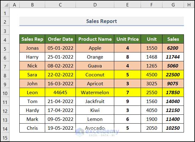
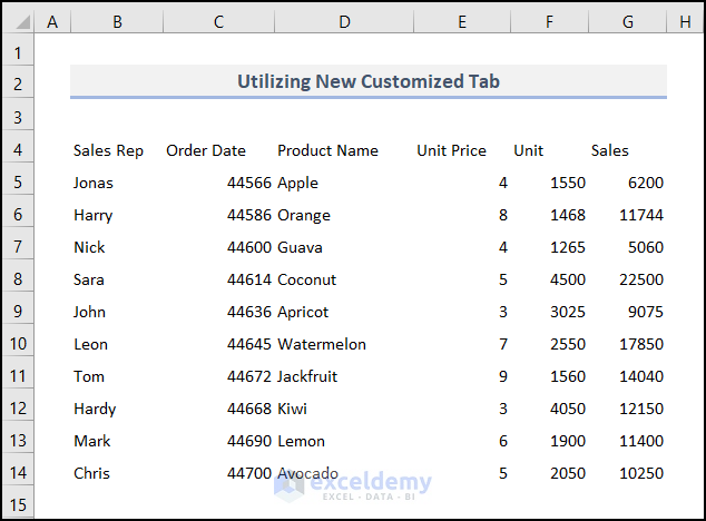
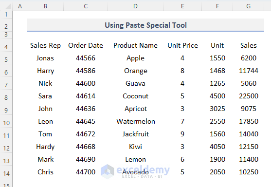
Here, we have a Sales Report for a particular month for a certain grocery store. This dataset includes the Sales Rep, Order Date, Product Name, Unit Price, Unit, and amount of Sales. As you can see the dataset is in a certain format. we are erasing the format with the Clear Formats command from the Home tab.
The Excel tutorial will cover:
- Use of the Clear button from the Home tab, Design tab, and Quick Access Toolbar (QAT) to remove formatting.
- Clearing the format of Excel Table and Pivot Table.
- Easy use of Format Painter and Paste Special tool to clear formatting.
- Application of VBA Macro for clearing formatting.
1. Using Clear Button from Home Tab to Clear Formatting in Excel
In the first approach, we’ll get the help of the Clear button existing in the Home tab ribbon to clear formatting in Excel. It’s simple & easy. Suppose, we have a Sales Report for a particular month for a certain grocery store. This dataset includes the Sales Rep, Order Date, Product Name, Unit Price, Unit, and amount of Sales in columns B, C, D, E, F, and G respectively. We will erase existing formatting with the Clear command.
Let’s check out the steps:
- At the very beginning, select cells in the B4:G14 range.
- Then, go to the Home tab.
- After that, click on the drop-down of the Clear button available in the Editing group.
- Next, select Clear Formats from the available options.
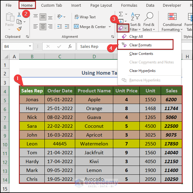
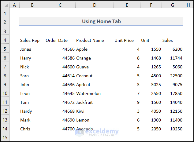
- Immediately, all the formatting gets gone from the worksheet.
2. Adding New Customized Tab to Clear Formatting in Excel
In our second method, we’ll create a new custom tab and a new group. Then, we’ll add the Clear Formats command to this group and use it. So, let’s explore it step by step.
📌 Steps:
- First of all, right-click on the Home tab. You can do the same on any other tab also.
- Secondly, click on Customize the Ribbon on the context menu.
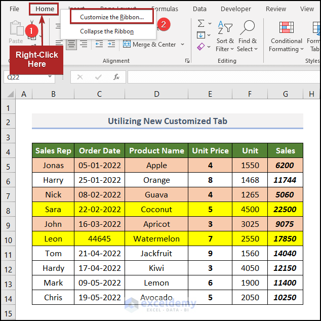
- Instantly, it opens the Excel Options window.
- At this time, press the New Tab button.
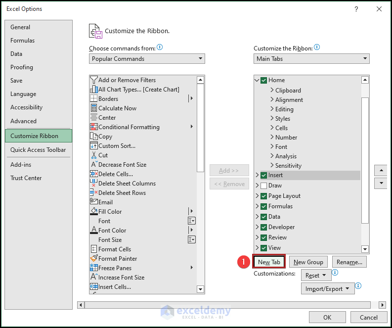
- This action creates a New Tab (Custom). See the image below.
![]()
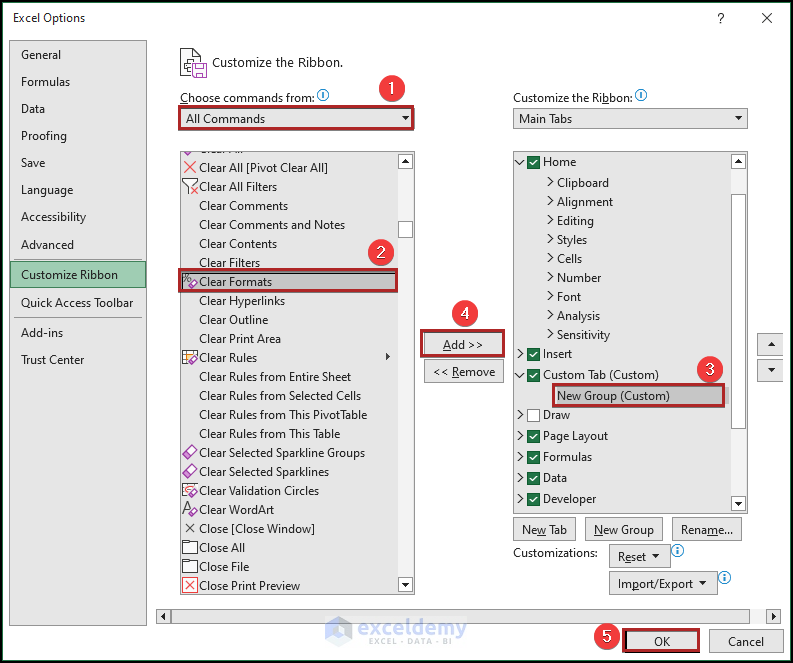
- Then, select All Commands from the Choose Commands from section.
- After that, scroll for the Clear Formats command and select it.
- Following this, select the New Group under the Custom Tab.
- Later, hit on Add >> button.
- Lastly, click OK.
- Presently, you can find the newly created Custom Tab beside the Insert tab. Also, the Clear Formats command is available under this tab on the New Group.
![]()
- Hence, select cells in the B4:G14 range.
- Therefore, move to the Custom Tab.
- After that, select the Clear Formats command.
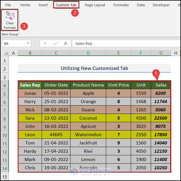
- Magically, you can see the worksheet without any formatting.
Read More: How to Clear Contents in Excel Without Deleting Formatting
3. Handling Excel Quick Access Toolbar (QAT) to Clear Formatting
In this method, we’ll add the Clear Formats command to the Quick Access Toolbar (QAT) and then use it to clear formatting in Excel. It’s a very quick and easy way to remove the formatting. So, let’s begin.
📌 Steps:
- At first, jump to the Home tab.
- Then, click on the Clear drop-down on the Editing group.
- After that, right-click on the Clear Formats command from the options.
- From the context menu, select Add to Quick Access Toolbar.
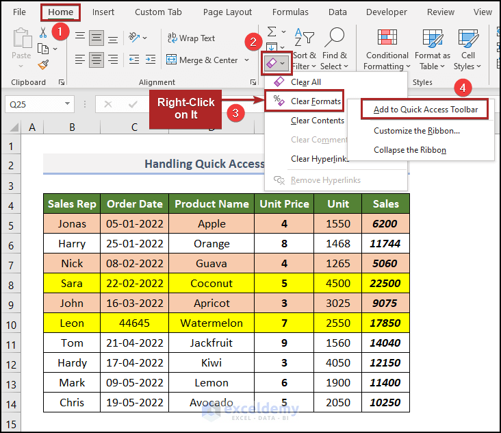
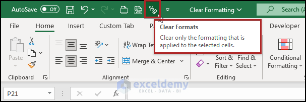
- Instantly, the command gets added to the QAT.
- Currently, select the whole B4:G14 range.
- Then, click on the Clear Formats command on the QAT.
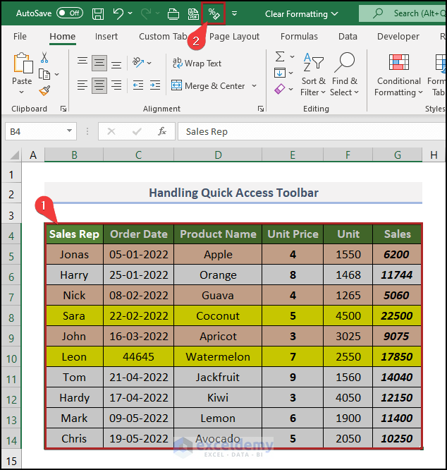
- And the result is before your eyes.
![]()
Read More: Difference Between Delete and Clear Contents in Excel
4. Clearing Formatting with Excel Format Painter Option
The Format Painter option helps us to copy the format of a selection and apply it to other content in the document. In this section, we’ll use this tool. Let’s explore the method step by step.
📌 Steps:
- Firstly, select a blank cell without any formatting. In this case, we selected cell A1.
- Secondly, proceed to the Home tab.
- Thirdly, click on the Format Painter tool on the Clipboard group.
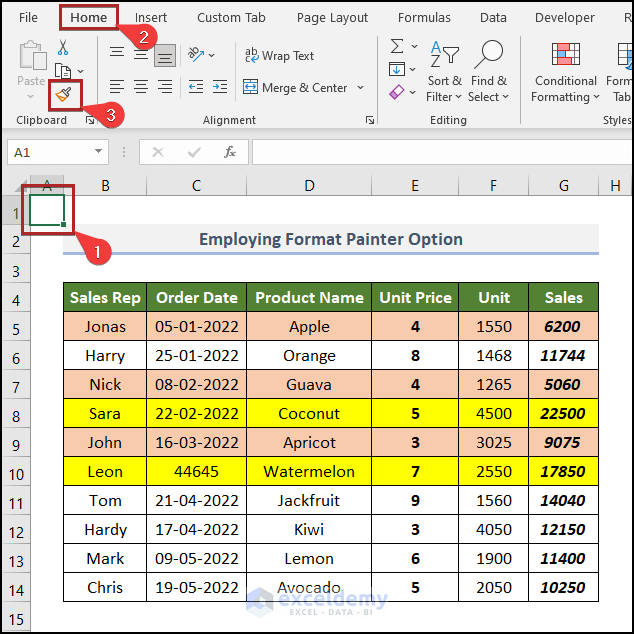
- Now, Format Painter has copied the format of cell A1. And the cursor takes the shape of a plus sign (+) and a paintbrush.
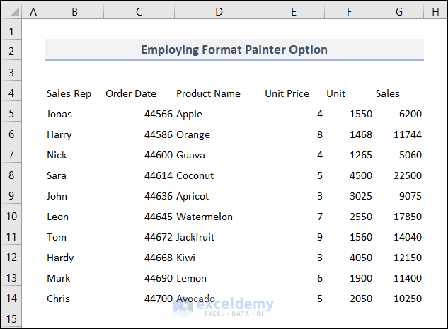
- Then, bring this cursor to cell B4 and click on it. After that, without releasing the click, drag it to cell G14 and then release it.
![]()
- Thus, our work is done.
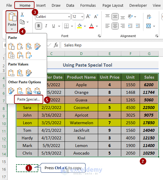
5. Using Excel Paste Special Tool to Clear Formatting
Now, we will clear formatting with the Paste Special tool in Excel. Please check the steps carefully.
📌 Steps:
- Select a blank cell B16 and copy it by pressing Ctrl + C keys.
- Then select the entire dataset.
- Then click as follows: Home => Paste => Paste Special.
- A Paste Special dialog box will appear. So, select Formats => OK.
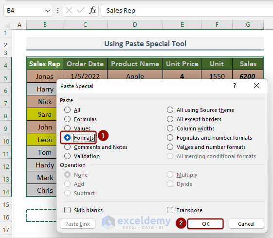
- Finally, we get the outcome after clearing the format.
6. Clearing Formatting by Applying Excel Keyboard Shortcut
Now, I know what you’re thinking. Are there any shortcut keys? Lucky you! There are shortcut keys to clear formatting in Excel. And this method describes just that.
📌 Steps:
- Firstly, select any cell inside the range B4:G14. Here, we selected cell B4.
- Secondly, press the CTRL key followed by A.
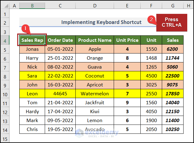
This action selects the whole range in a moment automatically.
- Then, press ALT + H + E + F simultaneously on the keyboard.
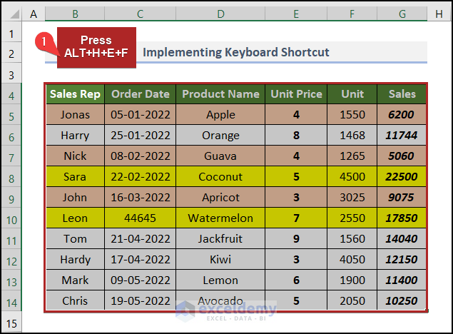
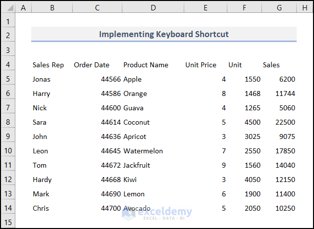
And, the formatting in the worksheet is gone.
7. Clearing Table Formatting in Excel with Quick Styles Command
Normally, when we insert a table in a spreadsheet, it appears with a banded row color format. One row gets a dark color, and its adjacent row gets a light color. This combination comes in default whenever we insert a table. Here is the table format of our previous dataset.
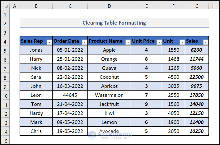
Now, we’ll show how we can clear this table formatting in Excel. So, stay with us.
📌 Steps:
- First and foremost, click on any cell inside the table. For example, we selected cell B5.
- Then, proceed to the Table Design tab.
- Therefore, click on the Quick Styles icon on the Table Styles group.
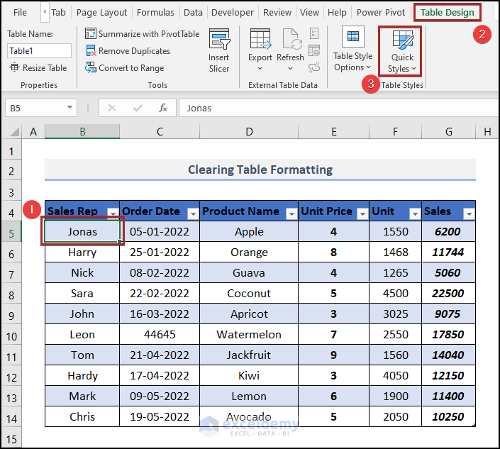
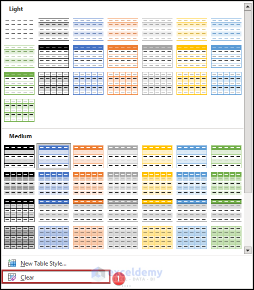
- Apparently, it opens a huge selection of table styles.
- But go to the bottom and select Clear.
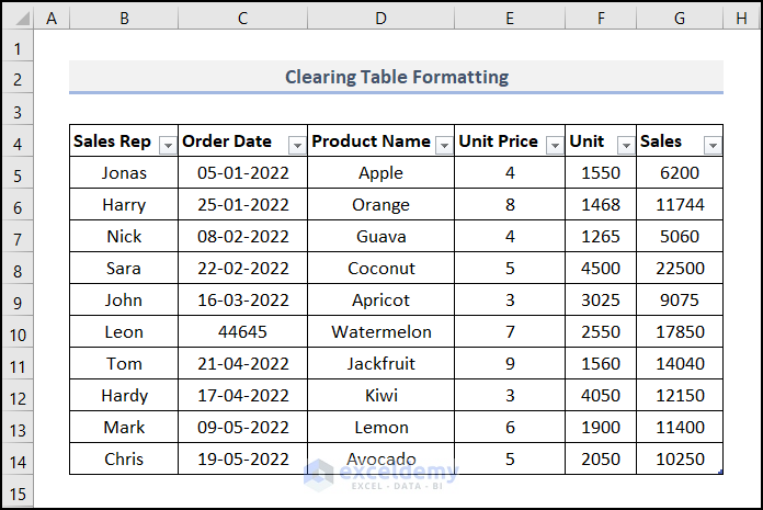
- Hence, this is still a table but without any formatting.
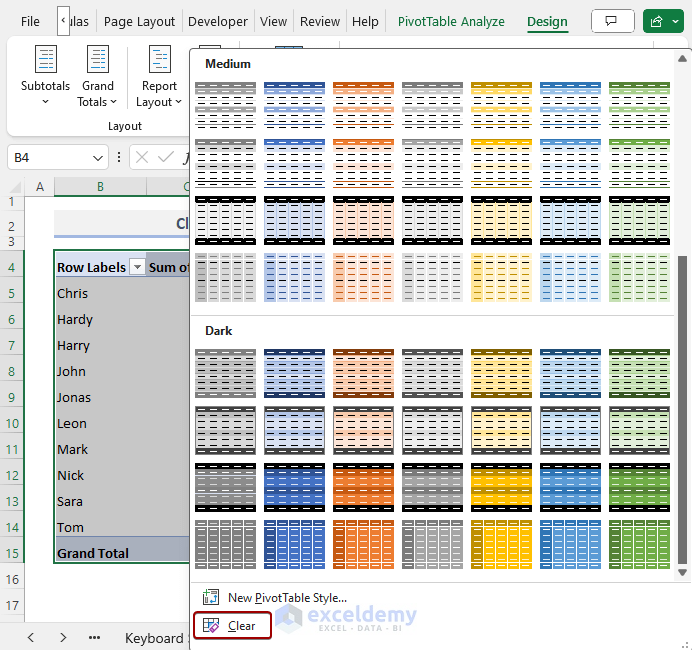
8. Clearing Formatting of Pivot Table Using Design Tab
In this section, we will learn how to clear the formatting of a Pivot Table in Excel with the Design tab. Therefore, the Pivot Table converts into a range.
📌 Steps:
- Select the pivot table and click as follows: Design => Quick Styles.
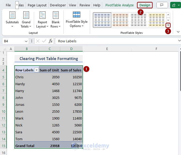
- Next, select the Clear command from the Quick Styles drop-down.
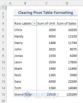
- As a result, Pivot table formatting is no longer visible and it converts into a range.
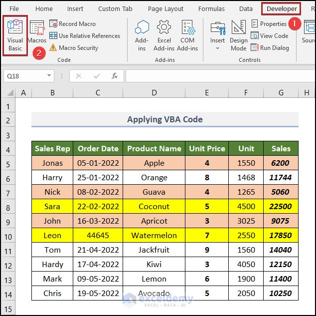
9. Applying VBA Macro to Clear Formatting
Have you ever thought of automating the same boring and repetitive steps in Excel? Think no more, because VBA has you covered. In fact, you can automate the prior method entirely with the help of VBA. Let’s see it in action.
📌 Steps:
- Initially, advance to the Developer tab.
- Then, click on Visual Basic in the Code group.
- Suddenly, the Microsoft Visual Basic for Applications window appears.
- Here, double-click on Sheet7(VBA) in the Project Explorer section.
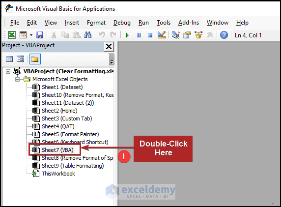
- Instantly, a code module opens on the right side.
- In this instance, copy the following code and paste them into the module.
Sub clear_format()
Worksheets("VBA").Range("B4:G14").ClearFormats
End Sub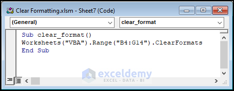
- Now, click on the green-colored play button on the ribbon. Actually, it’s the Run button. Also, you can press F5 on the keyboard to do the same.
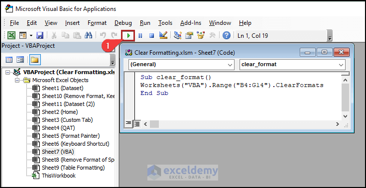
- Magically, the formatting gets removed from the worksheet.
![]()
Read More: How to Clear Cell Contents Based on Condition in Excel
How to Remove Automatic Formatting in Excel
When you enter data into a spreadsheet, Excel occasionally formats it automatically in a way that you didn’t expect. For instance, Excel will create a clickable link when you enter a web URL. Although this can be quite beneficial, there may be situations when you are opposed to it. If so, you can disable automatic formatting for a single cell or the entire workbook. Let’s see the process in detail.
📌 Steps:
- At the start, go to the File tab.
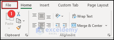
- Then, click on Options on the menu.
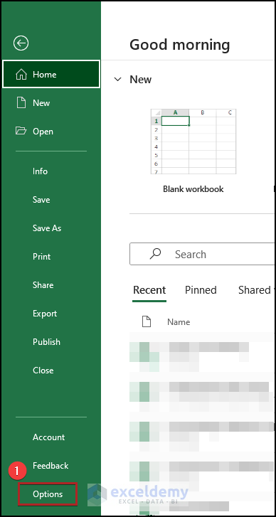
Immediately, the Excel Options window pops up.
- Here, move to the Proofing tab.
- After that, select the AutoCorrect Options… button.
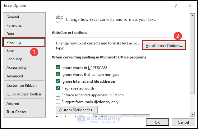
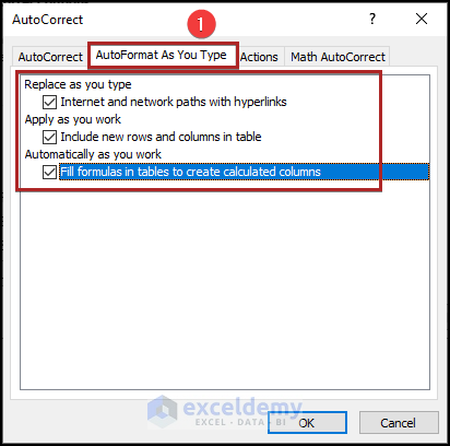
- Right away, the AutoCorrect dialog box appears.
- In the dialog box, go to the AutoFormat As You Type tab.
- Here, you can see three options. You can disable these options by unchecking the corresponding boxes.
How to Remove Formatting in Excel Without Removing Contents
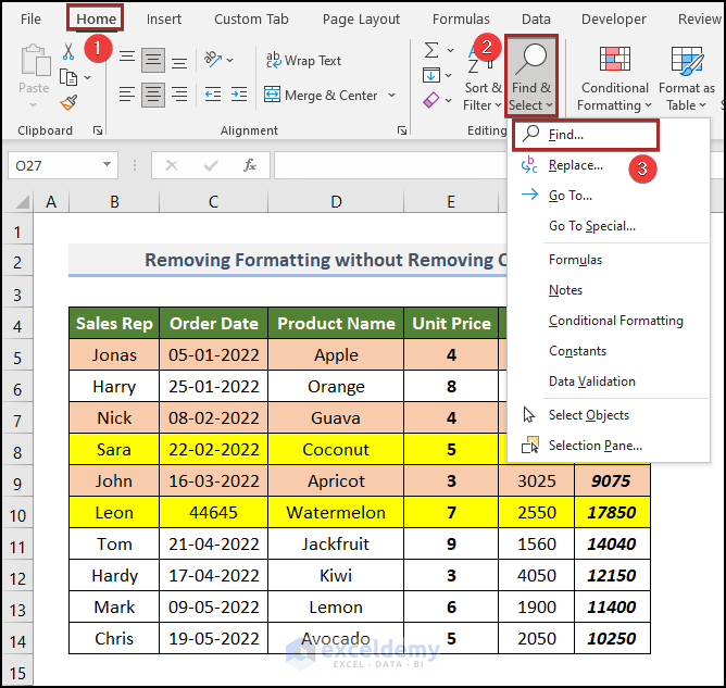
In the above dataset, we can see that rows 8 and 9 with sales greater than $15000 got the highlighting of yellow color. Here, we want to clear the formatting of just these two rows. Every other cell should be unchanged. How can we do that? See the following steps carefully.
📌 Steps:
- Primarily, move to the Home tab.
- Secondarily, click on the Find & Select drop-down on the Editing group.
- From the drop-down list, select the Find tool.
- Suddenly, the Find and Replace wizard appears.
- Then, click on the Format button.
![]()
It opens another new dialog box namely Find Format.
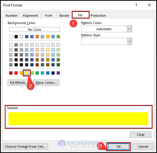
- Afterward, go to the Fill tab.
- From the available colors, choose Yellow (as it’s the background color of rows 8 and 10).
- Lastly, click OK.
- At this time, click on Find All button at the bottom of the Find and Replace wizard.
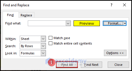
Here, we can see that this tool found 12 cells that match these criteria.
- Firstly, press CTRL + A to select all the cells in the list.
- Secondly, jump to the Home tab.
- Thirdly, click on the Clear drop-down icon.
- Lastly, choose the Clear Formats command.
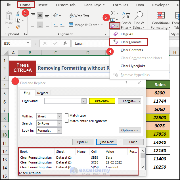
- Instantly, the formatting of these two rows vanishes.
![]()
Read More: How to Remove Formatting in Excel Without Removing Contents
How to Remove Table Formatting in Excel but Keep Data
Here, we’ll demonstrate how to clear table formatting but keep the data in Excel. So, without further delay, let’s dive in!
📌 Steps:
- In the first place, select cell B5.
- After that, go to the Table Design tab.
- In the Tools group, select the Convert to Range option.
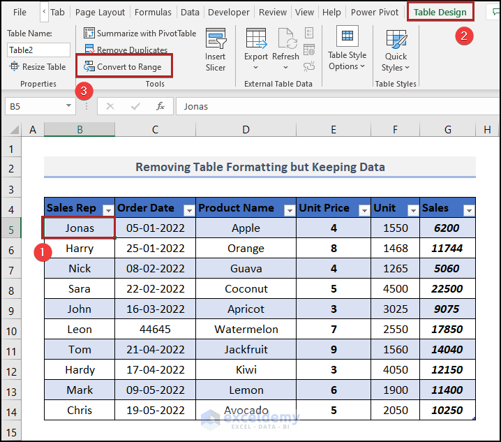
- In the MsgBox, choose Yes.
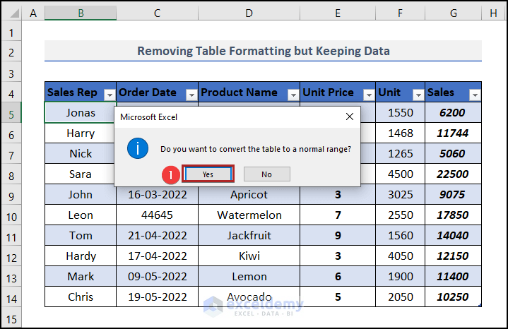
- Hence, it is now a simple data range rather than a table.
![]()
- Now, select the whole B4:G14 range.
- And clear the formatting like Method 1.
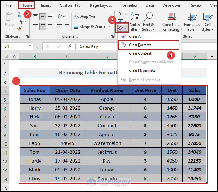
- And the final result is before your eyes.
![]()
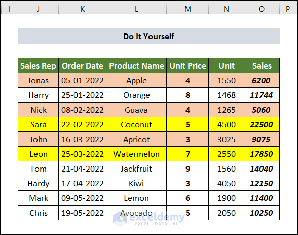
Practice Section
For doing practice by yourself we have provided a Practice section like the one below in each sheet on the right side. Please do it by yourself.
You may download the following Excel workbook for better understanding and practice yourself.
Conclusion
This article explains how to clear formatting in Excel simply and concisely. You can use the Clear button from the Home tab, Design tab, and Quick Access Toolbar (QAT) to remove formatting. However, you can also clear the format of Excel Table and Pivot Table. The Format Painter and Paste Special tools are useful for clearing formatting. Finally, the application of VBA Macro helps us to clear the formatting of multiple worksheets automatically.
Please let us know in the comment section if you have any queries or suggestions.
Related Articles
- How to Clear Excel Temp Files
- How to Clear Recent Documents in Excel
- How to Clear Multiple Cells in Excel
- How to Clear Cells with Certain Value in Excel
- How to Clear Contents in Excel Without Deleting Formulas
<< Go Back to Clear Contents in Excel | Entering and Editing Data in Excel | Learn Excel
Get FREE Advanced Excel Exercises with Solutions!

Nice work. But I have a sheet where i want to highlight the entire row with red color which sales is lesser than $15000 per month. But just the left cell os this row gets the formatting. Other not get changed. What can I do??
Hello DIALLO,
Thanks for your appreciation. I can get the problem you are facing with your worksheet.
Here, we have a dummy dataset in our hands to replicate your problem. It’s a Sales Report of a particular grocery store.
From the above dataset, we can clearly notice that there is a total of two sales that are greater than $15000, and others are less than this amount.
Now, we’ll show how you would do it in your workbook.
• At the very beginning, select cells in the B5:D14 range.
• After that, go to the Home tab.
• Then, click on the Conditional Formatting drop-down on the Styles group.
• Next, select New Rule from the list.
In the New Formatting Rule dialog box,
• At first, choose Use a formula to determine which cells to format under the Select a Rule Type section.
• Secondly, write down the following in the Format values where this formula is true box.
=D5<=15000• Thirdly, click on the Format button.
The Format Cells dialog box appears.
• Firstly, move to the Fill tab.
• Following this, select Red as Background Color.
• Later, click OK.
• Also, click OK in the New Formatting Rule dialog box.
Immediately, it shows us faulty formatting which we don’t want.
So, how can we fix it? Don’t worry! We just have to edit the formula.
To do this,
• Initially, proceed to the Home tab.
• Then, click on the Conditional Formatting drop-down.
• From the drop-down list, select Manage Rules.
Suddenly, it opens the Conditional Formatting Rules Manager.
• Primarily, select This Worksheet in the Show formatting rule for box.
• Secondarily, select the rule.
• Thirdly, click on Edit Rule.
• Change the formula a little bit. Just add a ($) sign before D5.
• Lastly, click OK.
• Again, click OK.
Now, you can see the correct formatting according to your preference.
That’s all from me on this. Keep the good vibes. You can follow our website Exceldemy, a one-stop Excel solution provider to explore more. Happy Excelling☕…..