Latest Posts From Musiha Mahfuza Mukta

What Is Delta E? Here, E represents “Empfindung”. Actually, Empfindung is a German word that means sensation. On the other hand, Delta is a Greek word that ...

Method 1 - Use Exponential Function POWER of Base 10 Steps: Select a blank cell C5 where you want to keep the exponents. Use the formula given below ...

When you have a large number as a cell value for monetary purposes, then you may need to abbreviate Billions in Excel. So, if you are looking for how to ...
Method 1 - Applying LEFT Function to Truncate Text in Excel Steps: Select a new cell D5 where you want to keep the result. You should use the formula ...
The following dataset contains three columns: Employee's Name, ID, and Tags. The Tags column contains three types of information. To find managers only: ...

Depreciation is a very common term in the case of assets. In general, it is the decline of an asset over a certain period of time. There are many methods to ...
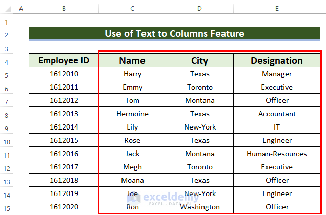
The sample dataset is given below where the column named Name City Designation has mixed information using multiple spaces. We want to separate the values. ...

Method 1 - Manually Creating a Fillable PDF Form Using Excel Step 1 - Create a Fillable Form Insert all the information that you want ...

If you are searching for how to look up a ZIP code for the name of a country or city in Excel, then you have come to the right place. Today, in this article I ...

Sometimes for data visualization, you may need to use an Excel chart. But when you hide your data, your chart may disappear. So, if you find the solutions to ...
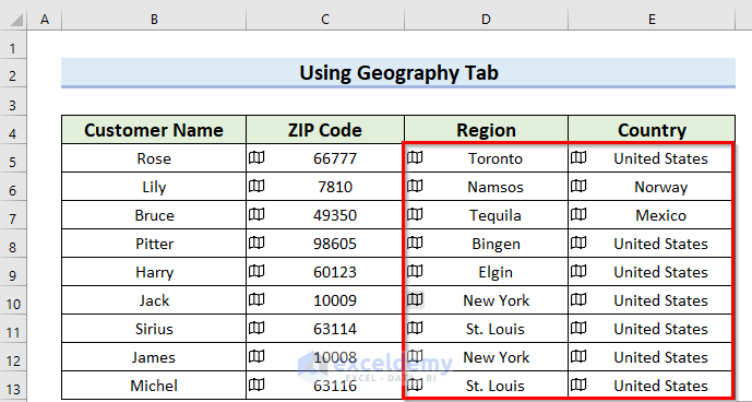
The below dataset contains 2 columns: Customer Name and ZIP Code. Method 1 - Using Geographic Data Type to Map Data by ZIP Code Steps: Select ...

Sometimes you may need to use the COUNTIF function between two values with multiple criteria. So, if you are looking for the use of a COUNTIF function between ...

Method 1 - Using Excel Translate Feature for Translating Japanese to English Steps: Open the Excel file containing the Japanese language data. Select ...
![[Fixed!] Iterative Calculation Not Working in Excel](https://www.exceldemy.com/wp-content/uploads/2022/11/7-Excel-Iterative-Calculation-not-Working.png?v=1697441998)
For research purposes, most of the time you may need to do an Iterative calculation. Sometimes, you may face the problem that you need to iterate but Excel is ...
![[Fixed] Excel Not Copying Formulas, Only Values (4 Solutions)](https://www.exceldemy.com/wp-content/uploads/2022/11/3-Excel-not-Copying-Formulas-only-Values.png?v=1697442137)
Copy-Paste is a very useful feature in Excel. Sometimes, you may face the problem that you need to copy the formulas along with the values or even only the ...
- « Previous Page
- 1
- 2
- 3
- 4
- 5
- …
- 7
- Next Page »
See Our Reviews at


Hello Daphne, the VBA code is perfectly working on my laptop. The code is fine. To run a VBA code you must follow:
1. Save your Excel file in .xlsm format
2. Use the Excel offline version
3. Enable macro content, to do so right click on Excel file >> from the Context Menu Bar >> go to Properties option >> General >> Security >> Unblock
Still, if you face the problem, then please go through this article [Fixed!] Macros Not Working in Excel. Hopefully, this article will help you to solve your issue.
Regards
Exceldemy Team
Thank you so much for pointing out this issue, Debbie! I wholeheartedly express my gratitude for the valuable time you dedicated to sharing your expertise and aiding others in addressing this matter.
I have added the limitations of Excel (regarding date format) in the article too. Thanks again!
Regards,
Musiha|Exceldemy
Hello, Sudhir, Thanks for your comment. You need to import external source data for Parish/County information. You can use the following link: u.s. census bureau’s website to get those information.
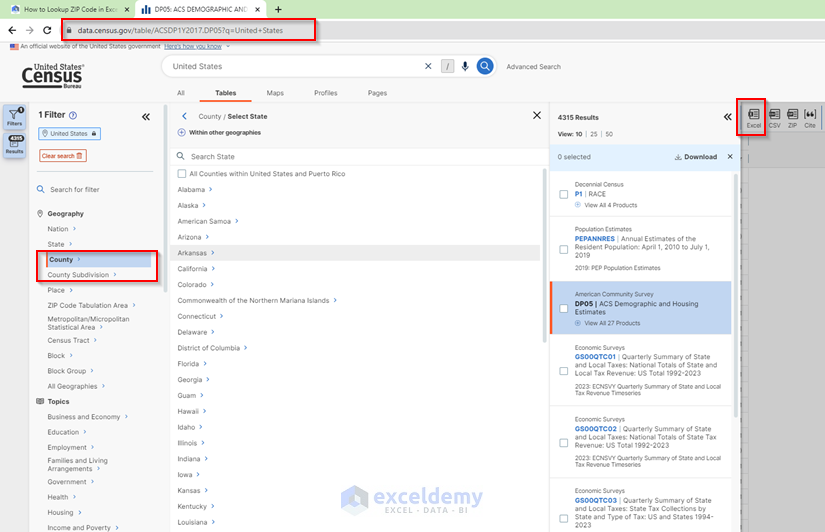
Also, this site provides the Excel file. So, you can download that file and use this as the source file.
Or, you can copy your needed data from this site and then paste these in your Excel file.
Regards
Musiha
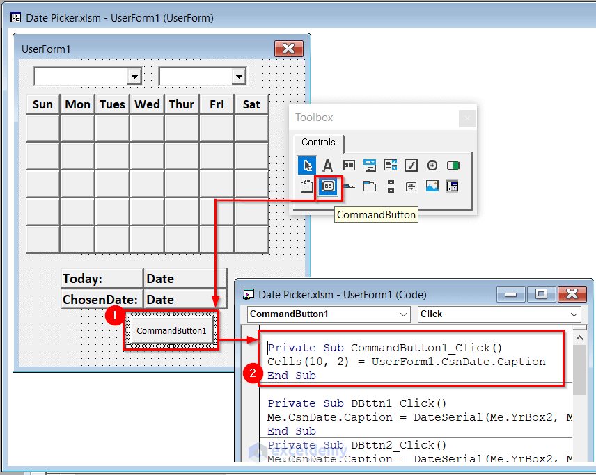
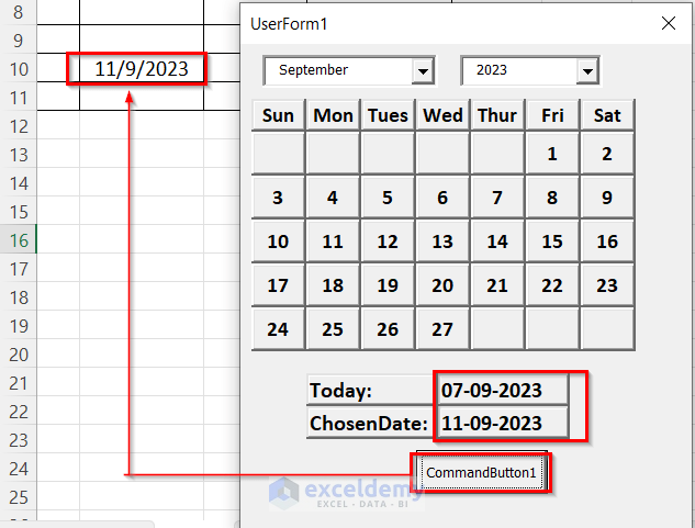
Thanks, IFN, for your comment. Here, the entire article explains how to create a Date Picker. But to get the drop-down menu, you should use more steps. So, after the completion of Date Picker, use the following steps.
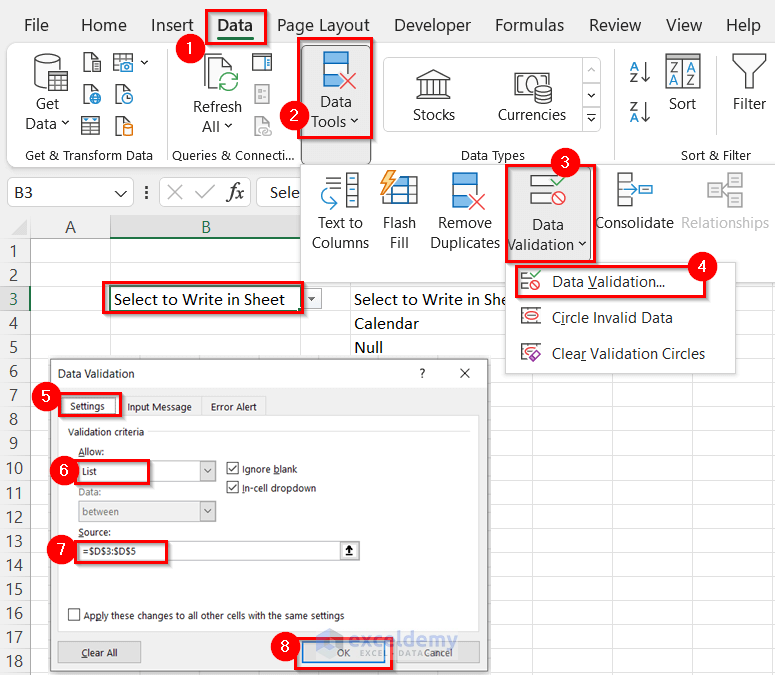
Step1: Select the cell where you want to keep the drop-down list >> from Data tab >> Data Tools group >> Data Validation >> Data Validation >> in the dialog box, go to Settings >> List >> Select range (the listed items including “Calendar” word) in the Source box >> press OK. As a result, you will get a drop-down list in that selected cell.
Step2: In the UserForm1, drag a new Command Button >> double click on Command Button >> write the following Code.
Use your preferred cell reference.
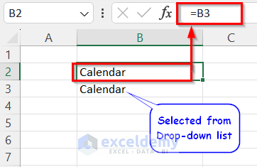
Step3: In B2 cell >> use this formula >> “=B3”
Step4: In VB Editor, from Insert tab >> Module >> write the following code in Module1.
Step5: Go to Worksheet >> right click on sheet name >> from Context Menu Bar >>View Code >> write the following code.
Step6: Now save the code >> go back to sheet >> check the output. When you choose “Calendar” from the dropdown list >> you will get the date picker visible >> choose your date >> press Command Button1 >> get the chosen date in B10 cell. If you get any error notice, then just press “End” to that notice.
When you selected the “Calendar” word, then with every change doing in your worksheet, you will get the date picker. So, if you need to write any other things, then first change the “Calendar” word from the drop down list.
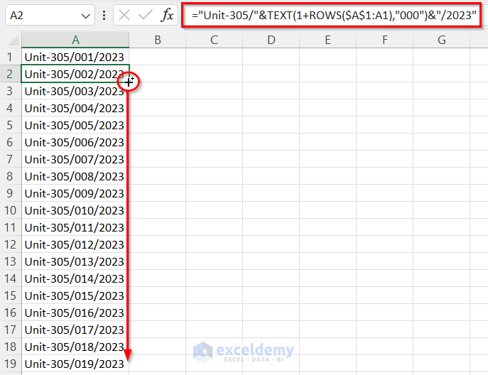
Hello Orly, to fill series with the middle number, you should use a formula. In A1 cell, keep the initial value. Then go to A2 cell >> use this formula–> =”Unit-305/”&TEXT(1+ROWS($A$1:A1),”000″)&”/2023″ >> press Enter. After that, drag the Fill Handle icon up to the last cell.
Formula Breakdown
After Equal Sign, write the first fixed part of your value within an Inverted Comma (“Unit-305/”). Then, use Ampersand Operator to join the formula. Here, inside the TEXT function use summation for the increment of middle number. Also, the TEXT function will consider the mentioned pattern (“001”).
Now, again give the Ampersand Operator, and within another Inverted Comma keep the last part of the value (“/2023”).
Regards
Musiha|Exceldemy
Hey Anita,
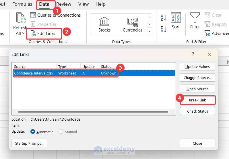
Sorry for the issues you are facing. If these methods don’t work, you can break the link to disable the updates. To break links, go to the Data tab >> select Edit Links >> select the link >> click on Break Link.
I hope this will help you solve the problem. Here, you can try some more options like changing the name of the Source file. Also, you should change the location of the Source file. It will stop Excel from connecting the existing file with the Source file.
Furthermore, if you don’t want to update your file, you can use the Copy-Paste(Value Only) feature for transferring data from a Source file.
Regards
Musiha|ExcelDemy
Thanks, Dennis, for your comment. You can use Format function of VBA to change the format. Below you can see I have changed the format of current date. The Format function will consider the expression and wanted format. Must use inverted commas for mentioning format.
Also, use this Format function in every command button to change the chosen date format.
For your better understanding, I’m mentioning the updated VBA code for new format.
You can see the result below.
Thank you Dave Gilblom, for your comment. Yes, Excel can do this. You should use some VBA codes for this. Below, I am attaching these codes.
–> In the Module 1 write the following code. Which will return the Sum of selected cells.
–> In the Module 2 write the following code. Which will return the Average of selected cells.
–> In the Module 3 write the following code. Which will return the Median of selected cells.
–> In the Module 4 write the following code. Which will return the standard deviation of selected cells.
–> Finally, in the ThisWorkbook >> write the following code.
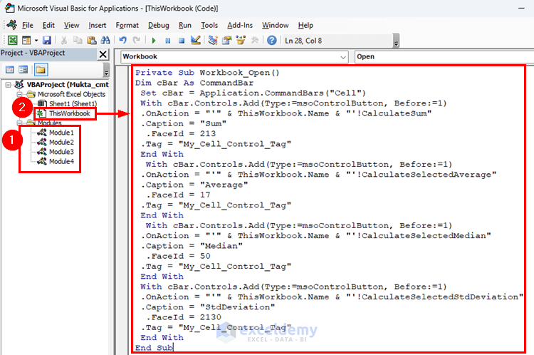
–> Now, save the code >> press on Run button >> close the Excel file >> re open the file >> select some cells >> right click >> from the Context Menu Bar.
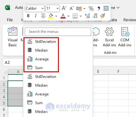
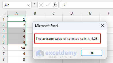
–> Then, choose the desire operation >> get the answer in MsgBox.
Thanks, KEVIN, for your suggestion. I have updated the article according to your concern. You may check it now.
Regards
Musiha | Team Exceldemy
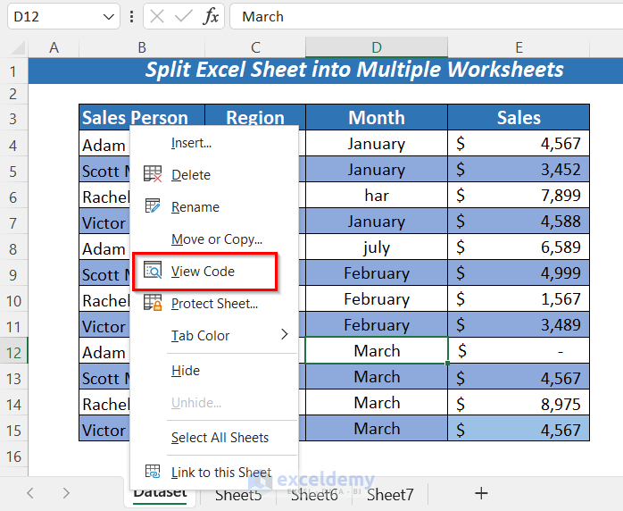
Thanks for your comment, Mojtaba. You can use VBA code which should be written in the original sheet. For example, I have a sheet named “Dataset“. I have divided this sheet into 3 sheets based on row. The names of these three sheets are Sheet5, Sheet6, and Sheet7. Now, write click on “Dataset” >> from the Context Menu Bar >> select View Code.
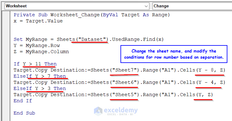
Write the following code in VB Editor.
Here, you must change the sheet names according to your workbook. Then you have to modify the conditions. Here, in my dataset there was 15 used rows. In the separated sheets there was 4 rows for each of them (except column headers). So, I set the conditions as row number > 11/7/3. So, when you change any cell value that value will be updated in the corresponding sheet. Like, if I change the cell value of C8 cell, then the change will be done in C4 cell of Sheet6 (as row number was 8).
So, set all the conditions properly for all sheets, then with any change of the original sheet, you will get the updated values in other sheet too.
Still, if you don’t get my point, then please comment or email us with the workbook. We will try to solve your problem.
Regards
Musiha/Exceldemy
Thank you, Salome for your comment. I’m very glad that you like the examples.
Now, come to your question. As my understanding, you need to create a custom list for sorting. In that list MARY should be kept at first. I have explained this in 1st method. You can check this. If you want anything else, please let us know in detail.
Thank you.
Thanks, Eliana Elia, for your comment. Step1: Select the cell where you want to keep the drop down list >> from Data tab >> Data Tools group >> Data Validation >> Data Validation >> in the dialog box, go to Settings >> List >> Select range (the listed items including “Calendar” word) in the Source box >> press OK. As a result, you will get a drop-down list in that selected cell.

Step2: In the UserForm1, drag a new Command Button >> double click on Command Button >> write the following Code.
Use your preferred cell reference.


Step3: In B2 cell >> use this formula >> “=B3”
Step4: In VB Editor, from Insert tab >> Module >> write the following code in Module1.
Step5: Go to Worksheet >> right click on sheet name >> from Context Menu Bar View Code >> write the following code.
Step6: Now save the code >> go back to sheet >> check the output. When you choose “Calendar” from the dropdown list >> you will get the date picker visible >> choose your date >> press Command Button1 >> get the chosen date in B10 cell. If you get any error notice, then just press “End” to that notice.
When you selected the “Calendar” word, then with every change doing in your worksheet, you will get the date picker. So, if you need to write any other things, then first change the “Calendar” word from the drop down list.
Thank you, Pankaj for your comment. Yes, there is no built-in process in Excel, but you can manually change the alignment of data labels. I have updated the article according to your comment. You can check the process.
Here you must use IFERROR function to get blank cell for null values. Again, you need to apply formula like if there is no data then the date will be blank also.
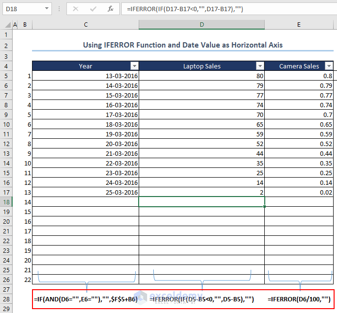
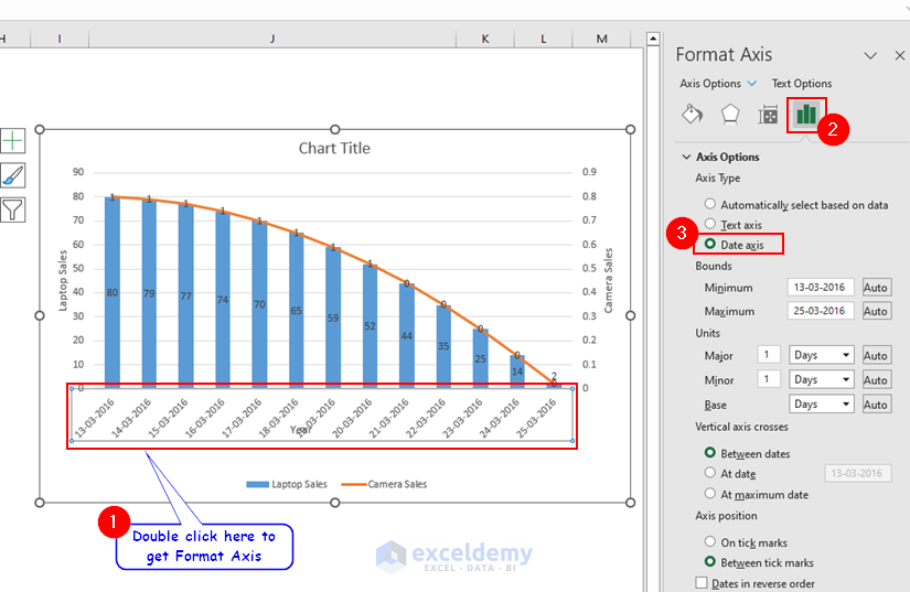
You must use Date format as Horizontal axis. Then you will get the chart auto updated up to valued cells. Double-click on Horizontal axis >> from Format Axis window (right side of Excel sheet) >> Axis Options >> Axis Type >> check Date axis.
Hello Daniel. You can do this by using the Find & Replace feature of Excel. From the Home tab >> under Editing group >> go to Find & Select option >> choose Replace. Then you will see the Find and Replace dialog box. Write 0 in Find what box >> write =NA() in Replace with box >> press in Find Next button >> if the cell has 0 value then press Replace button >> otherwise press Find Next.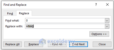
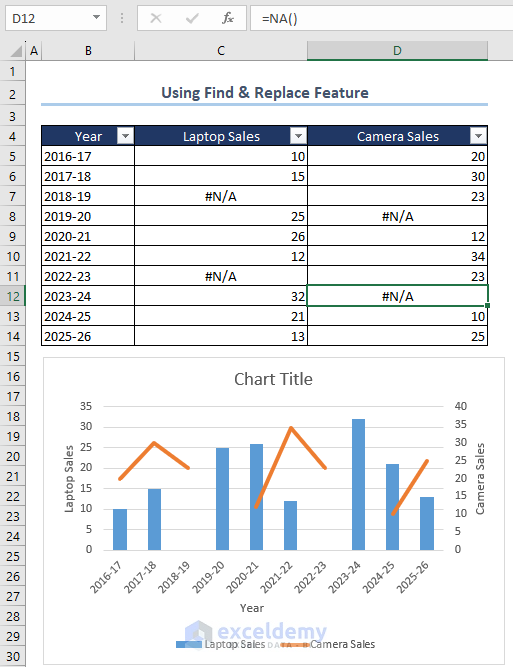
In this way change all the 0 values into =NA(). Don’t press Replace All as there may have numeric 0 with the numbers.
Now insert your chart. You will get both the axis have no zero values. Below, I have attached an image where I used two axis and remove zero value from both axis.
If you still face any problem then please provide us your worksheet in Exceldemy Forum.
Thank you, Bibhuti Sutar, for your comment. Here, you can hide the cells which you want to deselect. So, only the wanted values will be visible. In this case, you can use the following VBA code. For example, I used the given dataset. Here, I want to deselect/remove the cities named New York, Dallas, and California.
You must edit this according to the range. If it doesn’t work, then please inform us with more details in the reply or you can send us your workbook in Exceldemy forum.
Regards
Musiha Mahfuza|Exceldemy
Thank you, EAC for your comment. The possible solution is given below.
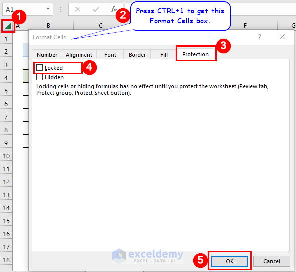
• Select all the cells by clicking the triangle where row and column headers coincide.
• Next, open the Format Cells by pressing Ctrl+1 >> Select the Protection option >> Uncheck the Locked option to unlock cells >> Click on OK.
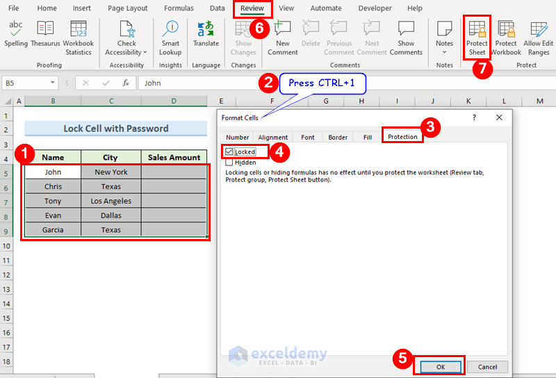
• Select the data range which you want to lock.
• Again, press Ctrl+1 >> The Format Cells dialog box will pop up >> Select Protection >> Next check on the Locked option >> Click on OK.
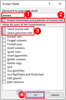
• Go to the Review tab in the ribbon >> Select Protect Sheet from the Protect group.
• A Protect Sheet dialog box will appear >> Set any password in the password box >> Check on the Protect worksheet and contents of locked cells>> Check both Select locked cells, Select unlocked cells.
• A Confirm Password dialog box will appear >> Rewrite your given password >> Click on OK.
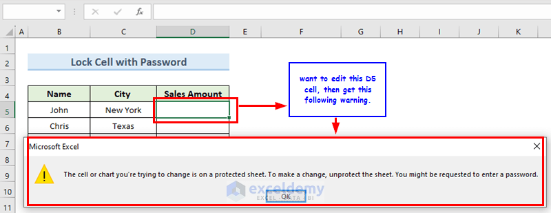
Now, try to edit the cells. Then you will get a warning from Microsoft Excel that you can’t change anything. To edit or enter any value, you have unprotected the Excel sheet with that password first.
Furthermore, you can see this article for more details How to Protect Excel Cells from Being Edited.
Thank you, CARLOS for your comment. You have to use the correct array (Sales Rep
or B5:B14) in INDEX function and Rank Column (D5:D14) in MATCH function. Also, while using the Fill Handle icon, you have to freeze both arrays. The most important part, you must write Rank 1,2,3.. manually in General format in F column.
There may have extra space or Apostrophe (‘) in the F column where you insert Rank numbers manually. You should remove all extra spaces.
You can see our article related MATCH function error. The link is: https://www.exceldemy.com/excel-match-function-not-working/#Case_1_NA_Error
For getting basic idea of INDEX-MATCH function you can see the examples from this article https://www.exceldemy.com/excel-index-match-example/
Still, you are facing the problem then please comment with your used formula and sample dataset.
Regards
Musiha Mahfuza Mukta| Team Exceldemy.
Thanks, KYLE, for your query. If there are identical values, then it will give same Rank. Also, the RANK function will skip one Rank. For your better understanding, I’m changing the sales value of Janifer to $9158. So, Zuschuss and Janifer get the same rank (2nd). Thus, the 3rd rank will be missed. Here, you must re-write the Rank of F7 cell to “2” and change the array for INDEX-MATCH function using in G7 an H7 cell. Basically, you need to set the array without Zuschuss information. Below, I have attached the whole scenario.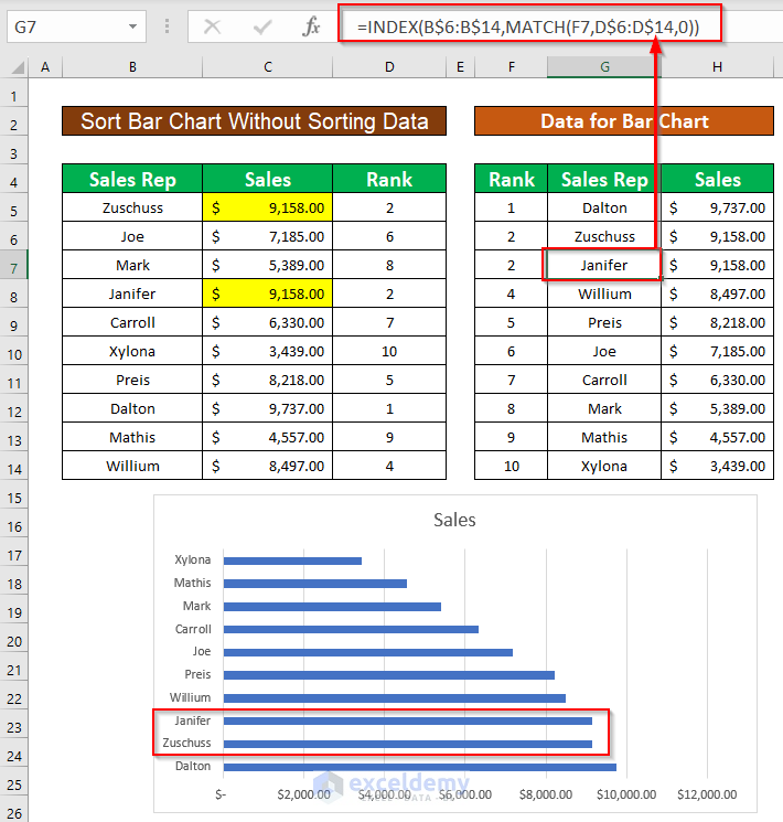
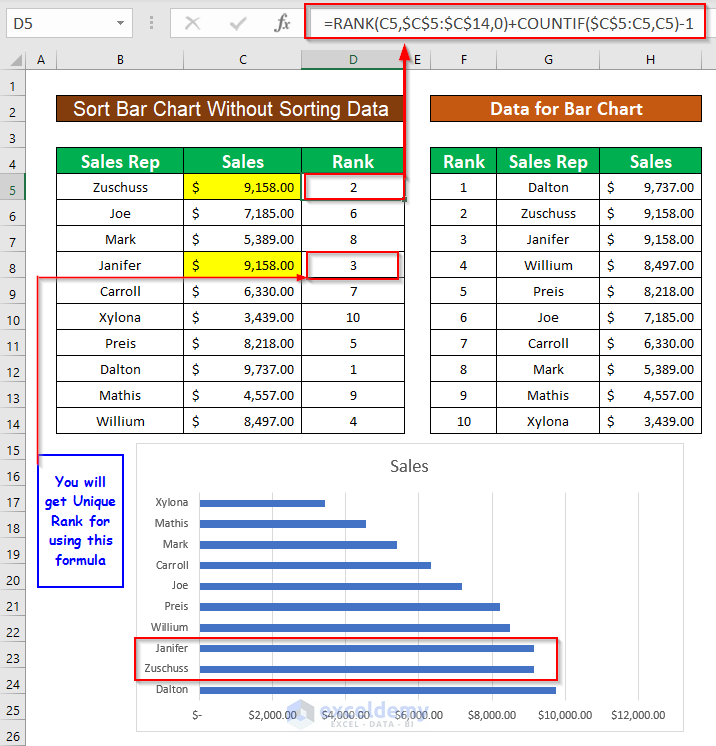
There is another way, if you want to get unique Rank for all. Like Zuschuss comes first than Janifer so Zuschuss will get 2nd rank and Janifer will get 3rd rank. In this case, you just need to change the formula in D column given below: =RANK(C5,$C$5:$C$14,0)+COUNTIF($C$5:C5,C5)-1
You don’t need to change the array of INDEX-MATCH function.
Regards
Musiha Mahfuza Mukta| Team Exceldemy
Hi ATIF, Thanks for your comment. Here, I made a dataset keeping the Text value in A column, Date value in B column and Counter will be in C column. If you provide your Excel file, then it will be more useful. As per my understanding, I am providing the following VBA code.
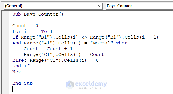
From Developer tab >> go to Visual Basic >> Insert a Module >> copy the code in that >> from Macros >> Run the code.
You can see the outcome below.
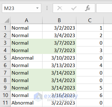
Where the counter counts single value for same date. I have highlighted the same date. Also, for “Abnormal” text the counter didn’t count.
In the code, you must mention total Row number of your dataset in For Next loop.
If you want only the text part, you can remove this portion
from code.
Hopefully this will work. If you are still facing problem, then please comment with more details or the sample dataset.
Regards
Musiha Mahfuza Mukta| Team Exceldemy
Thank you, MICHAEL KAIR for your comment. As per my understanding, there is no duplicate code. Actually, I have written the code part by part with detail description. Also, in the end, I have attached the complete code for making the Date Picker. That’s why, it seems to you the code is used twice but actually, the last one in Step 7 (last code) is the complete one. You should use only that one in your module. And the other codes are for explanation purpose.
I hope this will solve your problem. Please let us know if you face any further problems.
Regards,
Musiha Mahfuza Mukta,
ExcelDemy
Thank you ZOYSA for your comment. Below, I have attached two formulas for your problem.
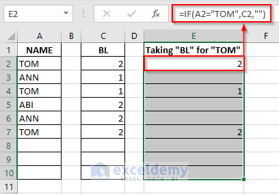
I have written the data from the A2 cell and C2 cell. According to your question, I have considered the dataset till A10 and C10.
Firstly, write the below formula in the E2 cell or the cell from where the NAME will be started.
=IF(A2=”TOM”,C2,””)
Then copy this formula up to E10 or your dataset’s end cell.
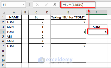
Then use another formula in the F4 cell.
=SUM(E2:E10)
Thank you PHUC YU for your comment. Actually, I have tried these methods too and the methods are working perfectly. Here, you can also zoom out the Excel file directly by clicking the Minus(-) sign situated right most corner of the file.
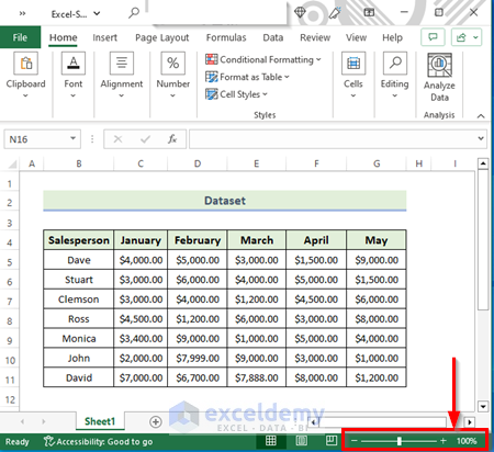
In case of, you are using an older version than 2013 of Excel then these methods may not work. Or, if you have any bugs or issues in your laptop then these would not work. I thing you were facing a different problem which is not related to this articles.
Thank you ROB for your comment. Here, ROW function is working as the row index number of the INDEX function. Actually, it should be ROW(B2:D9)=> {2;3;4;5;6;7;8;9} which denotes respectively the 2nd, 3rd, 4th…. up to 9th row number of this ($B$4:$D$12) array of INDEX function. Here, we ignore the 1st row of ($B$4:$D$12) this array as 1st row contains the Club Name’s not any player Name’s.
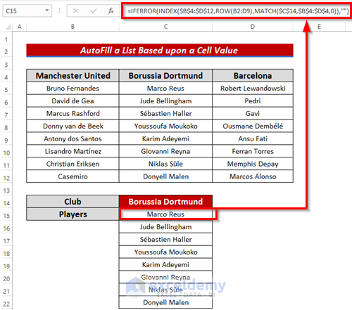
On the other hand, you have to use B4:D4 row in the MATCH function which will search for the Club Name’s and act as the column index number in the INDEX function.
Say, when you choose Borussia Dortmund or C4 cell from the list of C14 cell then the MATCH function will return 2 and thus the column index number of INDEX function will be 2 so INDEX function will give all the rows (except 1st one) of 2nd column of the given array which means all the player name’s of the Borussia Dortmund club.
So, you can use the formula like the below one. =IFERROR(INDEX($B$4:$D$12,ROW(B2:D9),MATCH($C$14,$B$4:$D$4,0)),””)
Hello MP ROY,
Thank you for your comment. I have tried these codes and they are working perfectly, except the code in Example3. For that particular code, you can use a new workbook. While I was using a new workbook the code has been perfectly worked there. But you have to be careful about the name of worksheet. You have to use exact worksheet number and name in the code.
Regards,
Musiha
Team ExcelDemy
Hello, J KUMAR.
Thank you for your comment. I have tried the code too and the code is absolutely right and perfectly working. But you are facing problem because most probably your device is running out of virtual memory. So, when you are trying this code in Excel, at that time you should close all other applications. Also, you should use an individual module for this code.
Hello, CHRIS.
Thank you for your comment. Actually, with the help of method 4, you are converting numbers into text. But when you re-entered any new value then the cell will hold that value excluding the apostrophe. Basically, the past value along with the apostrophe completely had gone away. So, if you want to keep the apostrophe then you should select that cell (containing new value) and run the Macros again. Then, you will see the apostrophe again with the new value.