The sample dataset has 4 columns: States, Product, Quantity, and Sales.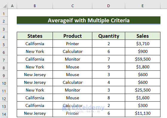
Method 1 – Applying AND & AVERAGEIF Functions for Multiple Criteria
Steps:
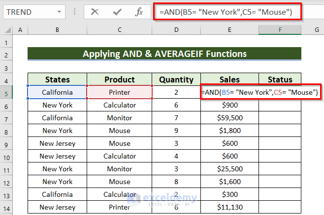
- Select a new cell, F5, where you want to keep the result.
- Enter the formula given below in the F5 cell:
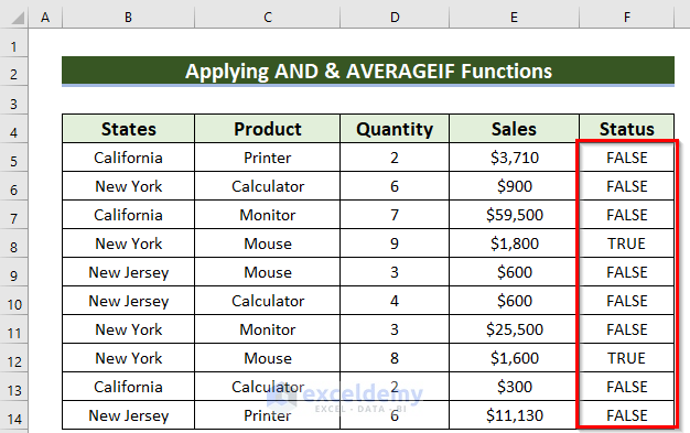
=AND(B5= "New York",C5= "Mouse")In this formula, the AND function will return TRUE if the cell value of B5 is “New York” and the cell value of C5 is “Mouse.”
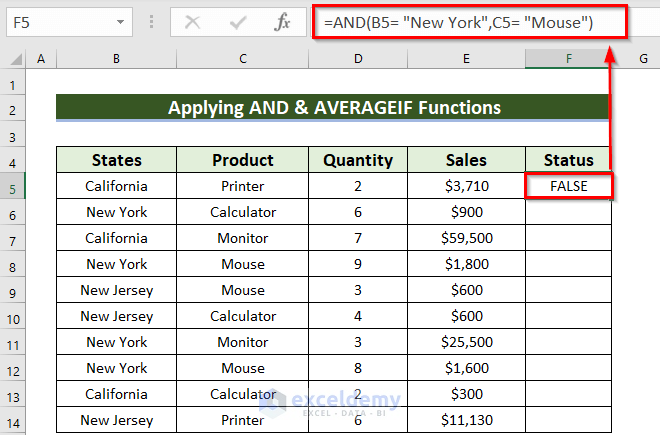
- Press ENTER to get the result.
- Drag the Fill Handle icon to AutoFill the corresponding data in the rest of the cells F6:F14. Or you can double-click on the Fill Handle icon.
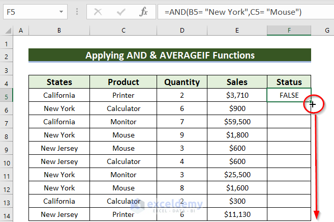
You will get the Status. This means you will come to know whose cells fulfill that logic.
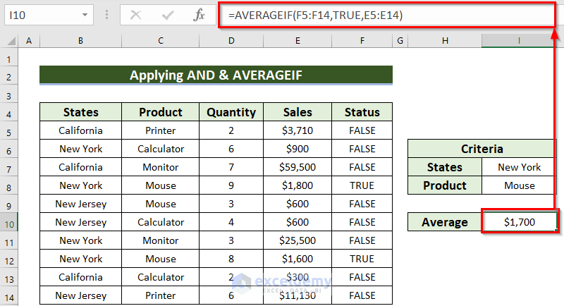
- Enter the following formula in the I10 cell:
=AVERAGEIF(F5:F14,TRUE,E5:E14)Here, in this formula, the AVERAGEIF function will do the average of the Sales column because E5:E14 is the average range. Additionally, F5:F14 is the criteria range, and TRUE is the criteria.
- Press ENTER.
You will get the average sales for the product Mouse from New York.
Read More: How to Calculate Average If Number Matches Criteria in Excel
Method 2 – Using the AVERAGEIF Function & OR Logic
Steps:
- Select a new cell, F5, where you want to keep the result.
- Enter the formula given below in the F5 cell:
=AVERAGE(AVERAGEIF(C5:C14,"Mouse",E5:E14),AVERAGEIF(C5:C14,"Calculator",E5:E14))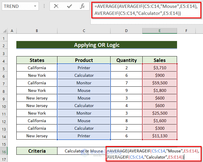
Formula Breakdown
- Firstly, AVERAGEIF(C5:C14,”Calculator”,E5:E14)—> here the AVERAGEIF function will average from the E5:E14 data range, which will fulfill the given condition. In addition, the condition is in the C column, whose cell value is Calculator.
- Output: $600.
- Secondly, AVERAGEIF(C5:C14,”Mouse”,E5:E14)—-> again the AVERAGEIF function will average from the E5:E14 data range, which will fulfill the given condition. In addition, the condition is in the C column, the cell value of which is Mouse.
- Output: $1333.
- Lastly, AVERAGE($600,$1333)—> returns $967.
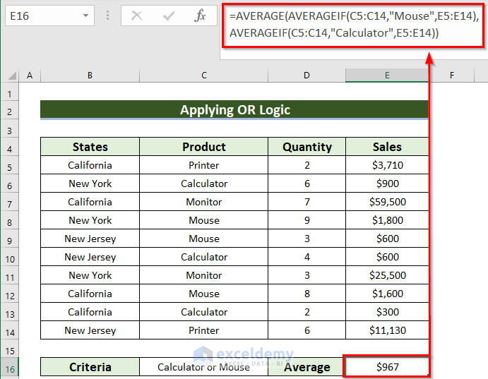
- Press ENTER to get the result.
You will get the average Sales for the product Calculator or Mouse.
Method 3 – Employing the AVERAGEIF Function with Multiple Criteria
Steps:
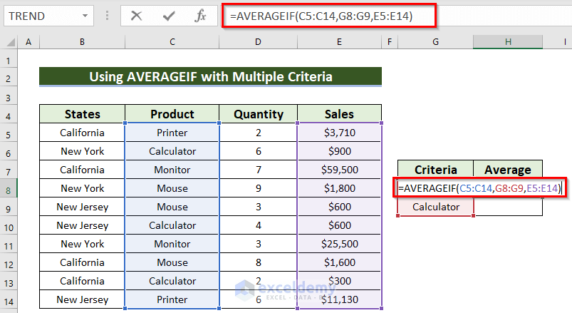
- Enter the criteria in cells G8:G9.
- Select a new cell, H8, where you want to keep the result. Here, you should keep blank cells next to cell H8. The blank cells should be equal to the number of given criteria.
- Enter the formula given below in cell H8:
=AVERAGEIF(C5:C14,G8:G9,E5:E14)Here, the AVERAGEIF function will average from the E5:E14 data range, fulfilling the given condition. Additionally, C5:C14 is the criteria range, and G8:G9 is the criteria.
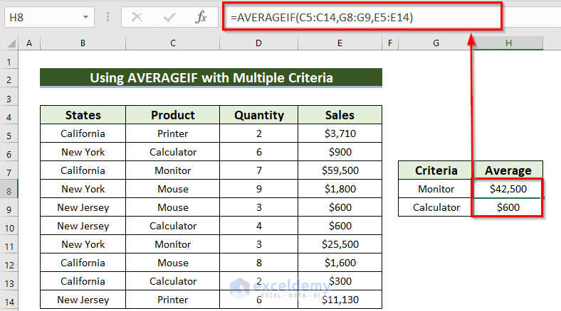
- Press ENTER to get the result.
You will get the average sales individually for the Monitor and Calculator products.
Calculate the average output.
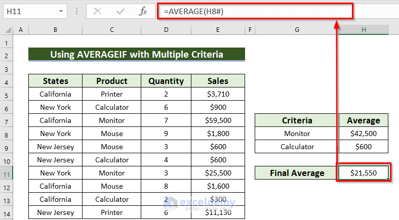
- Enter the following formula in cell H11:
=AVERAGE(H8#)In this formula, the AVERAGE function will calculate the average of the H8 and H9 cells. The Hash (#) sign appears when only two cells are in a data range.
- Press ENTER.
You will get the average sales for the Monitor and Calculator products.
Read More: Excel AVERAGEIF with ‘Greater Than’ and ‘Less Than’ Criteria
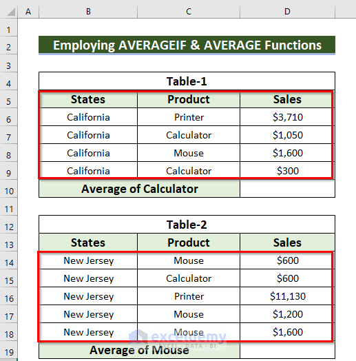
Method 4 – Employing AVERAGE & AVERAGEIF Functions
We have the following dataset, which has two tables.
Steps:
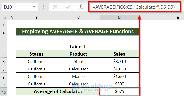
- Select a new cell, D10, where you want to enter the result.
- Enter the formula given below in cell D10:
=AVERAGEIF(C6:C9,"Calculator",D6:D9)Here, in this formula, the AVERAGEIF function will calculate the average of the Sales column because D6:D9 is the average range. Additionally, C6:C9 is the criteria range, and Calculator is the criteria.
- Press ENTER.
You will see the average Sales for the product Calculator from the state of California.
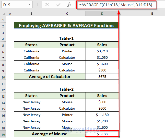
Let’s find the average sales for the Mouse product from New Jersey.
- Select a new cell, D19, where you want to enter the result.
- Enter the formula given below in cell D19:
=AVERAGEIF(C14:C18,"Mouse",D14:D18)Here, in this formula, the AVERAGEIF function will calculate the average of the sales column because D14:D18 is the average range. Additionally, C14:C18 is the criteria range, and Mouse is the criteria.
- Press ENTER.
You will see the average sales for the Mouse product from New Jersey.
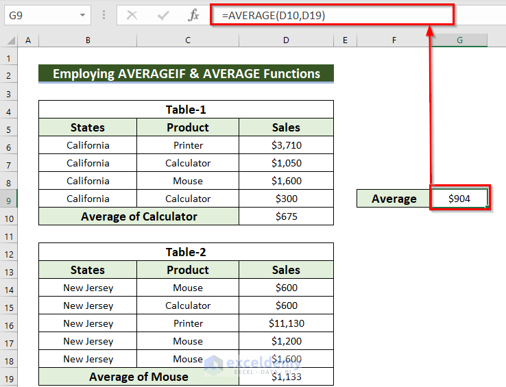
Find the final average.
- Enter the following formula in cell G9:
=AVERAGE(D10,D19)In this formula, the AVERAGE function will do the average of the D10 and D19 cells.
- After that, press ENTER.
Finally, you will get the average sales for the product Calculator from the state of California and the Mouse from the state of New Jersey.
Read More: How to Find Average If Values Lie Between Two Numbers in Excel
Method 5 – Using the AVERAGEIF Function in Array
Steps:
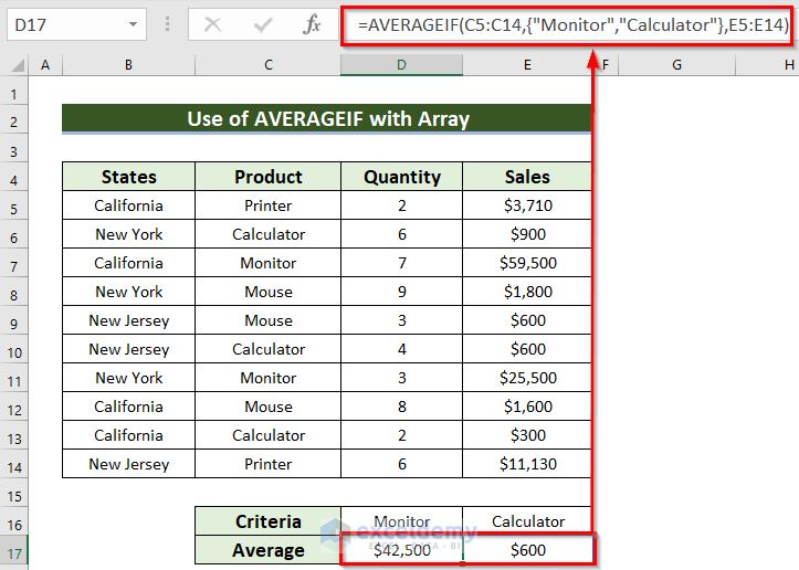
- Select a new cell, D17, where you want to keep the result. Here, you should keep blank cells next to cell D17 (horizontally). The blank cells should be equal to the number of given criteria.
- Enter the formula given below in cell D17:
=AVERAGEIF(C5:C14,{"Monitor","Calculator"},E5:E14)Here, the AVERAGEIF function will average from the E5:E14 data range, fulfilling the given condition. Additionally, C5:C14 is the criteria range, and the criteria are Monitor and Calculator.
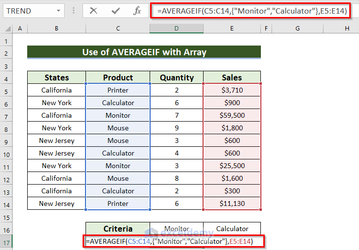
- Press ENTER to get the result.
You will get the average sales individually for the Monitor and Calculator products.
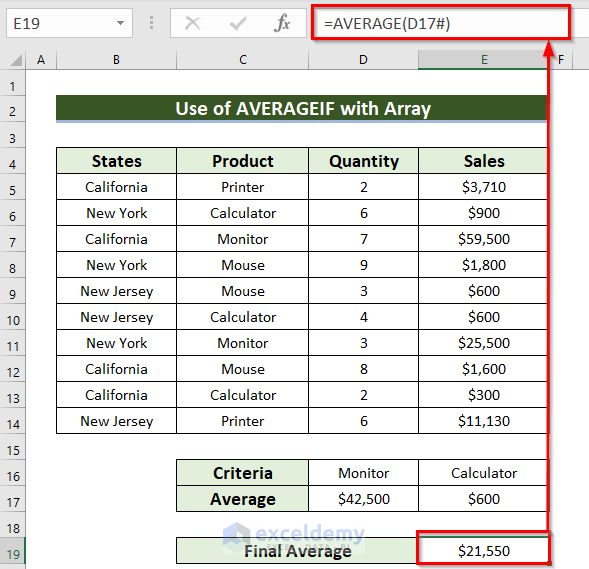
Calculate the average of the output.
- Enter the following formula in cell E19:
=AVERAGE(D17#)In this formula, the AVERAGE function will do the average of the D17 and E17 cells. The Hash (#) sign appears when only two cells are in a data range.
- Press ENTER.
You will get the final sales average for the Monitor and Calculator product.
Read More: Excel AVERAGEIF Function for Values Greater Than 0
Use of the AVERAGEIFS Function in Excel
Steps:
- Select a new cell, H10, where you want to keep the result.
- Enter the formula given below in cell H10:
=AVERAGEIFS(E5:E14,B5:B14,"California",C5:C14,"Mouse")- Press ENTER.
You will get the average sales for Product: Mouse from States: California.
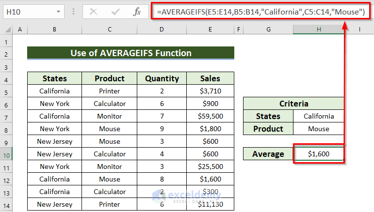
Formula Breakdown
Here, the AVERAGEIFS function will average from the E5:E14 data range, fulfilling the given condition.
- Firstly, B5:B14 is the 1st criterion range, and “California” is the criteria.
- Secondly, C5:C14 is the 2nd criteria range and “Mouse” is the criteria.
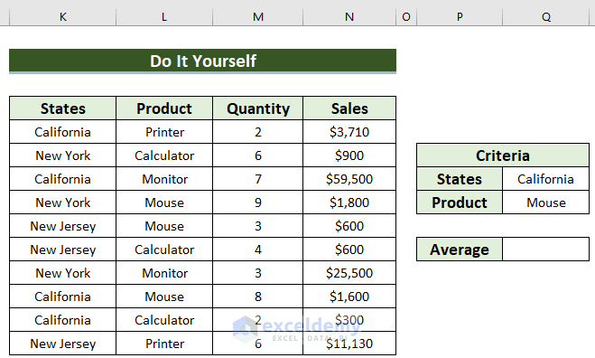
Practice Section
Now, you can practice the methods.
Download the Practice Workbook
You can download the practice workbook from here:
Related Articles
- How to Find Average If Cell Contains Text in Excel
- How to Calculate Average If Cell Is Not Blank in Excel
<< Go Back to Excel AVERAGEIF Function | Excel Functions | Learn Excel
Get FREE Advanced Excel Exercises with Solutions!
