In our daily lives, calculating the average of cells containing specific text is a typical chore, and this is where Microsoft Excel shines. In the following article, we’ll outline 4 approaches how to find average if cell contains text in Excel. Moreover, we’ll also go through how we can compute the average of cells that do not contain a particular text.
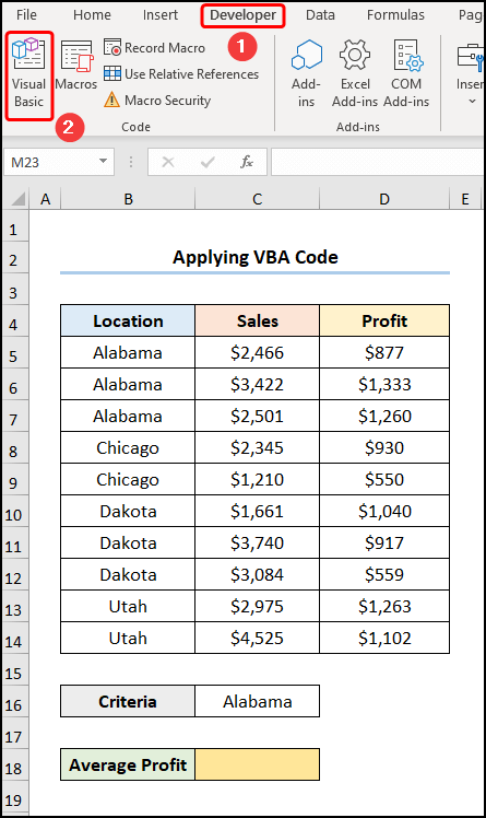
Now, let’s consider the Sales and Profit based on the Location dataset shown in the B4:D14 cells which shows the Location, Sales, and Profit in USD respectively. Henceforth, let us glance at each of the methods shown below with simple illustrations.
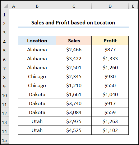
Here, we have used Microsoft Excel 365 version, you may use any other version according to your convenience.
Method-1: Calculate the Average in Excel If Cell Contains Text (Single Criterion)
Let’s start with the simplest way to obtain the average based on a single text criterion. In simple terms, we want to enter the name of a Location and calculate the corresponding Average Sales made according to the dataset. Therefore, let’s take a close look at the following three sub-methods.
1.1 Using AVERAGEIF Function
Firstly, let’s familiarize ourselves with the AVERAGEIF function which computes the arithmetic mean of the cells specified under a given condition or criterion. Here, we’ve chosen Chicago as the Criteria and we want to obtain the Average Sales, so, just follow these steps.
📌 Steps:
- At the very beginning go to the C18 cell >> enter the formula given below.
=AVERAGEIF(B5:B14,C16,C5:C14)
Here, the B5:B14 and C5:C14 range of cells refer to the Location and Sales columns respectively and the C16 cell represents the Criteria Chicago.
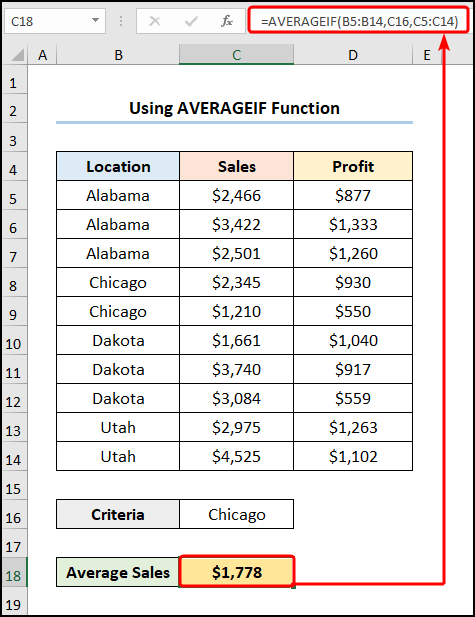
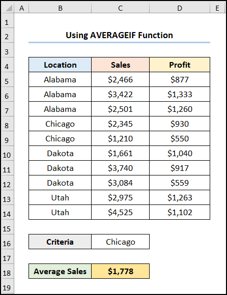
Finally, the results should look like the image given below.
1.2 Use of AVERAGEIFS Function
The AVERAGEIFS function is similar to the AVERAGEIF function with the added benefit that it handles multiple criteria from different rows and columns to return the average value. In this case, we’ve chosen only one Criterion which is Chicago, and we want to calculate the Average Sales, hence, just follow along.
📌 Steps:
- Initially, move to the C18 cell >> type in the formula shown below.
=AVERAGEIFS(C5:C14,B5:B14,C16)
In the above expression, the B5:B14 and C5:C14 range of cells indicate the Location and Sales columns whereas the C16 cell represents the Criteria Chicago.
Formula Breakdown:
- AVERAGEIFS(C5:C14,B5:B14,C16) → finds average for the cells specified by a given set of conditions or criteria. Here, C5:C14 is the average_range argument which is the Sales column. Next, B5:B14 is the criteria_range1 argument which refers to the Location column and the C16 is the criteria1 argument which is Chicago.
- Output → $1778
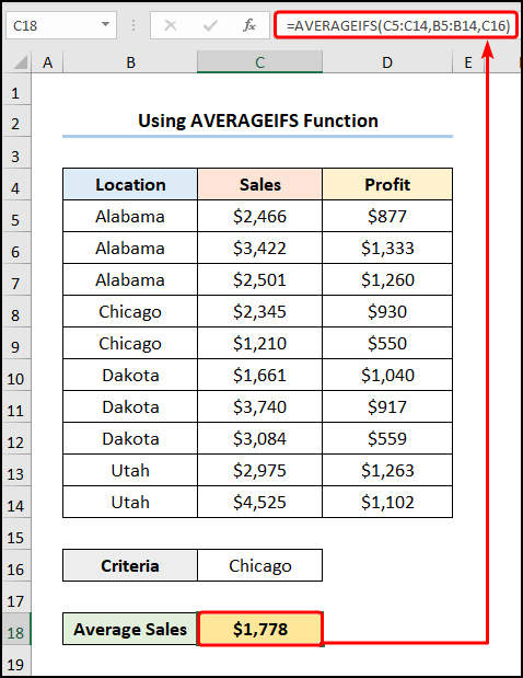
Lastly, your output should look like the picture shown below.

1.3 Applying Excel VBA Code
Alternatively, you can also calculate the average based on a single text criterion using the VBA Code below. It’s simple & easy, just follow along.
📌 Steps:
- First, navigate to the Developer tab >> click the Visual Basic button.
Now, this opens the Visual Basic Editor in a new window.
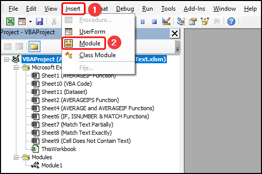
- Second, go to the Insert tab >> select Module.
For your ease of reference, you can copy the code from here and paste it into the window as shown below.
Sub Calculate_Average_with_Condition()

Dim wrksht As Worksheet
Set wrksht = Worksheets("VBA Code")

wrksht.Range("C18") = Application.WorksheetFunction. _
AverageIf(wrksht.Range("B5:B14"), wrksht.Range("C16"), _
wrksht.Range("D5:D14"))

End Sub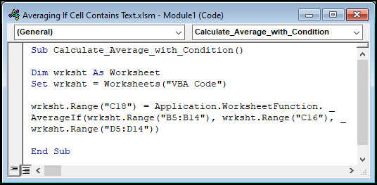
⚡ Code Breakdown:
Now, I will explain the VBA code which is divided into 2 steps.
- In the first portion, the sub-routine is given a name, here it is Calculate_Average_with_Condition().
- Next, define the variable wrksht and assign the “VBA Code” worksheet to this variable.
- In the second potion, specify the cell where to return the result using the Range object, in this case, the C18 cell.
- Now, use the WorksheetFunction object to call the AVERAGEIF function.
- Following this, specify the range argument which is the B5:B14 range, the criteria argument which is the C16 cell, and finally, the average_range argument which is the D5:D14 range.

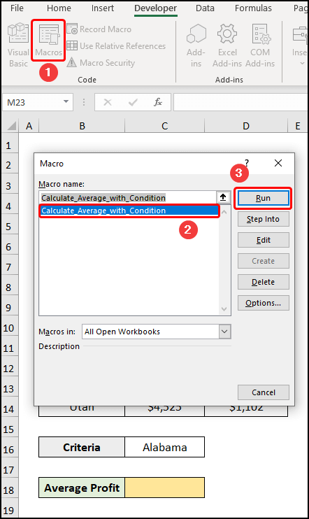
- Third, close the VBA window >> click the Macros button.
This opens the Macros dialog box.
- Following this, select the Calculate_Average_with_Condition macro >> hit the Run button.
Eventually, the results should look like the screenshot shown below.

Read More: Excel AVERAGEIF with ‘Greater Than’ and ‘Less Than’ Criteria
Method-2: Finding Average If Cell Contains Text (Multiple Text Criteria)
What if you want to specify more than one condition? In the following sub-methods, we’ll answer this exact question by selecting two text criteria to calculate the average value. So, let’s see it in action.
2.1 Using AVERAGE and AVERAGEIF Functions
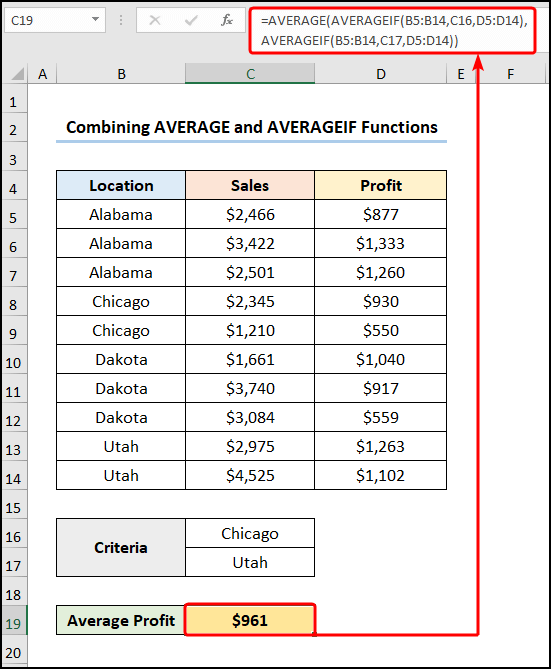
In this sub-method, we’ll combine the AVERAGE and AVERAGEIF functions to compute the Average Profit for the given Locations of Chicago and Utah.
📌 Steps:
- In the first place, navigate to the C19 cell and insert the following expression in the Formula Bar.
=AVERAGE(AVERAGEIF(B5:B14,C16,D5:D14),AVERAGEIF(B5:B14,C17,D5:D14))
In the above formula, the B5:B14 and D5:D14 range of cells point to the Location and Profit columns while the C16 and C17 cells refer to the Criteria of Chicago and Utah.
Formula Breakdown:
- AVERAGEIF(B5:B14,C16,D5:D14) → returns the arithmetic average for the cells specified by a given set of conditions or criteria. Here, B5:B14 is the range argument which is the Location column. Next, C16 is the criteria argument that refers to Chicago. Following this, D5:D14 is the average_range argument which refers to the Profit column.
- Output → $740
- AVERAGEIF(B5:B14,C17,D5:D14) → In this expression, the C16 cell is the criteria argument that refers to Utah while the B5:B14 and D5:D14 ranges refer to the Location and Profit columns.
- Output → $1183
- AVERAGE(AVERAGEIF(B5:B14,C16,D5:D14), AVERAGEIF(B5:B14,C17,D5:D14)) → becomes
- AVERAGE(740, 1183) → returns the average of the arguments. Here, the values of 740 and 1183 are summed and divided by 2 to return their respective average.
- Output → $961
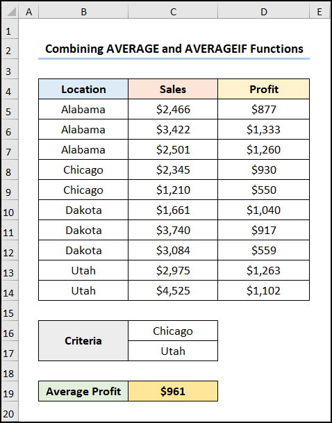
Subsequently, the result should look like the image given below.
2.2 Combining Excel IF, ISNUMBER, and MATCH Functions
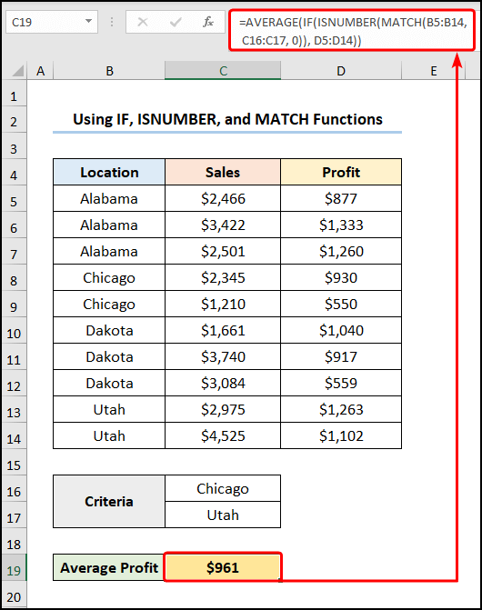
As another option, you can also utilize the IF, ISNUMBER, and MATCH functions to calculate the Average Profit using two conditions which are Chicago and Utah. Now, allow me to demonstrate the process in the steps below.
📌 Steps:
- To begin with, jump to the C19 cell and enter the following expression.
=AVERAGE(IF(ISNUMBER(MATCH(B5:B14,C16:C17, 0)), D5:D14))
In this formula, the B5:B14, C16:C17, and D5:D14 ranges represent the Location, Criteria, and Profit.
Formula Breakdown:
- MATCH(B5:B14,C16:C17, 0) → returns the relative position of an item in an array matching the given value. Here, B5:B14 is the lookup_value argument which refers to the Location. Following, C16:C17 represents the lookup_array argument that is the value to be matched. Lastly, 0 is the optional match_type argument which indicates the Exact match criteria.IF(ISNUMBER(MATCH(B5:B14,C16:C17, 0)), D5:D14)
- IF(ISNUMBER(MATCH(B5:B14,C16:C17, 0)), D5:D14) → checks whether a condition is met and returns one value if TRUE and another value if FALSE. Here, ISNUMBER(MATCH(B5:B14,C16:C17, 0)) is the logical_test argument which returns only the matched values from the Profit column D5:D14 (value_if_true argument) otherwise it returns blank (value_if_false argument).
- AVERAGE(IF(ISNUMBER(MATCH(B5:B14,C16:C17, 0)), D5:D14)) → becomes
- AVERAGE(930, 550, 1263, 1102) → returns the average of the arguments. Here, the values of 930, 550, 1263, and 1102 are summed and divided by 4 to return their respective average.
- Output → $961
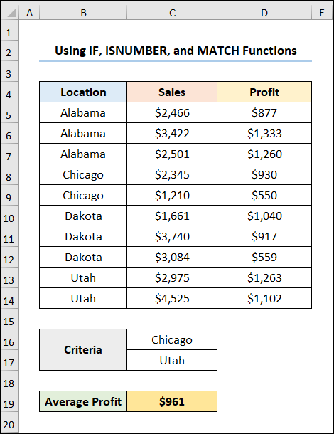
Consequently, your output should look like the picture given below.
Read More: How to Find Average If Values Lie Between Two Numbers in Excel
Method-3: Averaging Cells That Match Text Exactly
Another way to match text with the AVERAGEIF function involves using the Wild Card Character. For instance, we want to find the Average Sales in the Location which have the letters “ta” present in the name. Therefore, just follow the steps shown below.
📌 Steps:
- To start, proceed to the C18 cell and type in the formula given below.
=AVERAGEIF(B5:B14,"*ta*",C5:C14)
In the above formula, the B5:B14 and C5:C14 range of cells refer to the Location and Sales columns respectively while “*ta*” represents the Criteria. As a note, the Asterisk(*) character before and after tells the function to look for the keyword within a string of text. In this case, it matches all instances of the Locations Dakota and Utah.
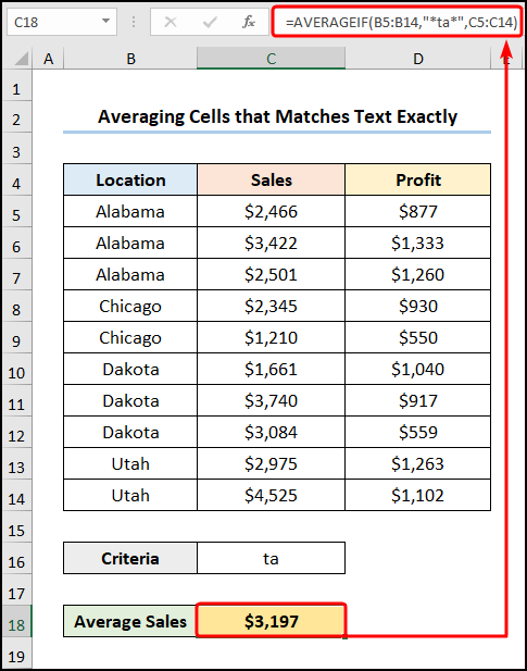
Consequently, your output should appear as the image given below.

Read More: How to Calculate Average If Number Matches Criteria in Excel
Method-4: Find the Average of Cells That Match Text Partially
In a similar manner, we can use the Wild Card characters to get the Average Sales for the Location which partially matches the letters “ta”. Hence, let’s see the procedure in detail.
📌 Steps:
- First and foremost, go to the C18 cell and insert the expression given below.
=AVERAGEIF(B5:B14,"*ta",C5:C14)
Here, the Asterisk(*) character before the keyword tells the function to look for those instances ending with “ta” which matches all the occurrences of Location Dakota.
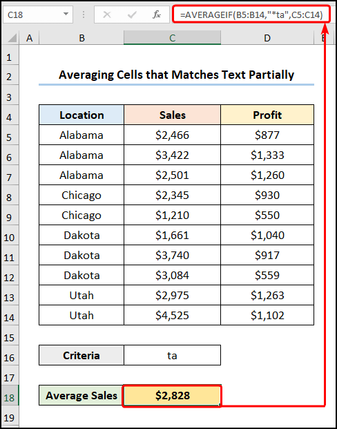
Finally, the result should look like the screenshot given below.

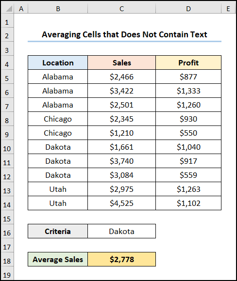
How to Calculate Average If Cell Does Not Contain Text in Excel
So far we’ve discussed how to find average if cell contains text in Excel, but you can also exclude certain strings of text using the AVERAGEIF function. In this instance, we want to exclude the text Dakota and calculate the Average Sales for the rest of the Locations. So, let’s see the process step-by-step.
📌 Steps:
- Initially, copy and paste the following expression into the C18 cell as shown below.
=AVERAGEIF(B5:B14,"<>*Dakota*",C5:C14)
In the above formula, the <> character is the Not Equal to operator which instructs the function to exclude all the instances of the text Dakota when calculating the Average Sales. In this case, all of the Locations except Dakota are matched.
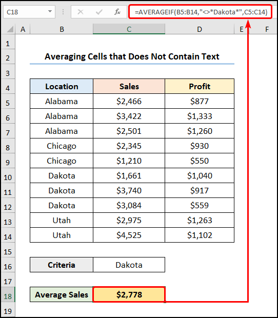
Eventually, the Average Sales should be equal to the value of $2778.
Download Practice Workbook
You can download the practice workbook from the link below.
Conclusion
In this article, we’ve shown you 4 effective methods for how to find average if cell contains text in Excel. I suggest you read the full article carefully and apply the knowledge to your needs. You can also download our free workbook to practice. I hope you find this article helpful and informative. If you have any further queries or recommendations, please feel free to comment here.
Related Articles
- Excel AVERAGEIF Function for Values Greater Than 0
- How to Calculate Average If Cell Is Not Blank in Excel
- How to Use Excel AVERAGEIF with Multiple Criteria
<< Go Back to Excel AVERAGEIF Function | Excel Functions | Learn Excel
Get FREE Advanced Excel Exercises with Solutions!
