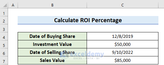
The sample dataset contains two columns with Investment Details.
Method 1 – Using a Generic Formula to Calculate the ROI Percentage
Steps:
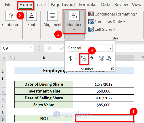
- Select C9 to display the calculated ROI percentage.
- In the Home tab, go to Number.
- Choose Percentage (%).
- Select C9 and enter the formula:
=(C7-C5)/C5C7 contains the Sales value and C5 the Investment value.
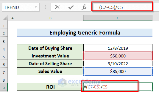
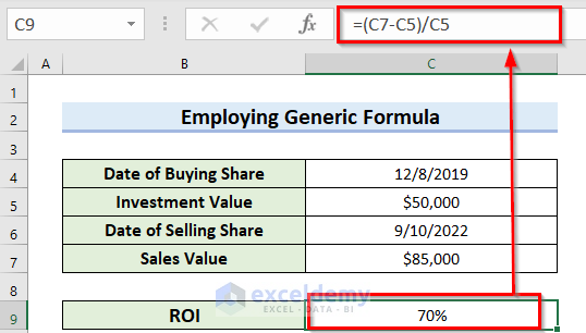
- Press ENTER.
You will see the ROI percentage:
Method 2 – Calculating ROI Percentage of Capital Gain in Excel
Steps:
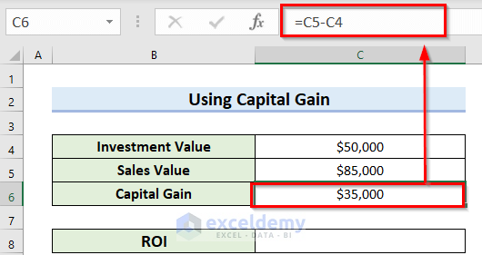
- Select C6 to find the Capital Gain.
- Use the formula in C6.
=C5-C4C5 cell contains the Sales Value and C4 the Investment Value.
- Press ENTER.
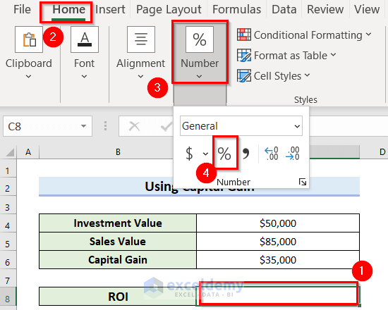
- Select C8 cell to see the calculated ROI percentage.
- In the Home tab, go to Number.
- Choose Percentage (%).
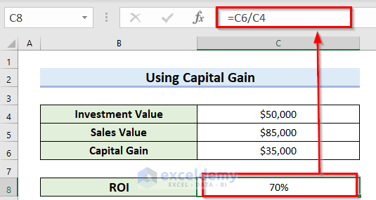
- Select C8 to calculate the ROI percentage and enter the formula:
=C6/C4C6 cell contains the Capital gain and C4 the Investment Value.
- Press ENTER.
You will see the ROI percentage.
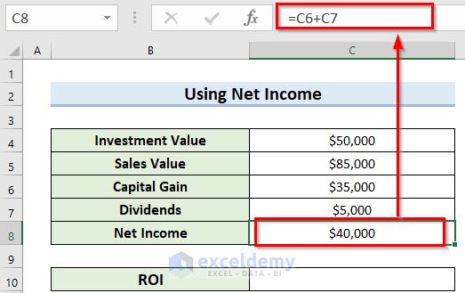
Method 3 – Calculating the ROI Percentage using the Net Income in Excel
Steps:
- Select C6 to find the Capital Gain.
- Use the formula in C6.
=C5-C4C5 contains the Sales Value and C4 the Investment Value.
- Press ENTER.
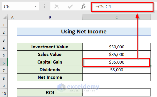
You will get the value of the Capital Gain.
- Select C8 to see the Net Income and use the following formula:
=C6+C7C6 contains the Capital Gain and C7 cell the Dividends value.
- Press ENTER.
You will see the value of the Net Income.
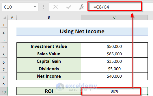
- Select C10 to calculate the ROI percentage and use the formula:
=C8/C4C8 contains the Net Income and C4 the Investment value.
- Press ENTER and convert the result into percentage using the Number format in the Home tab.
You will see the ROI percentage:
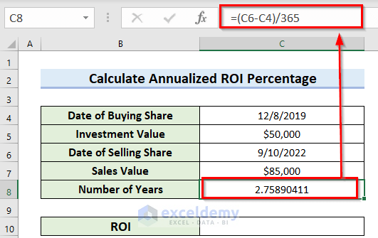
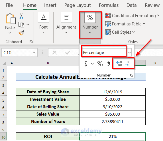
Method 4 – Calculating the ROI Percentage for the Annual Return in Excel
Steps:
- Select C9 to keep the Number of Years.
- Use the formula in C9.
=(C6-C4)/365C6 cell contains the Date of Selling Share and C4 the Date of Buying Share. By subtracting the two dates you will get the total days in between. You must divide the result by 365 to find the number of years.
- Press ENTER.
You will get the total Number of Years.
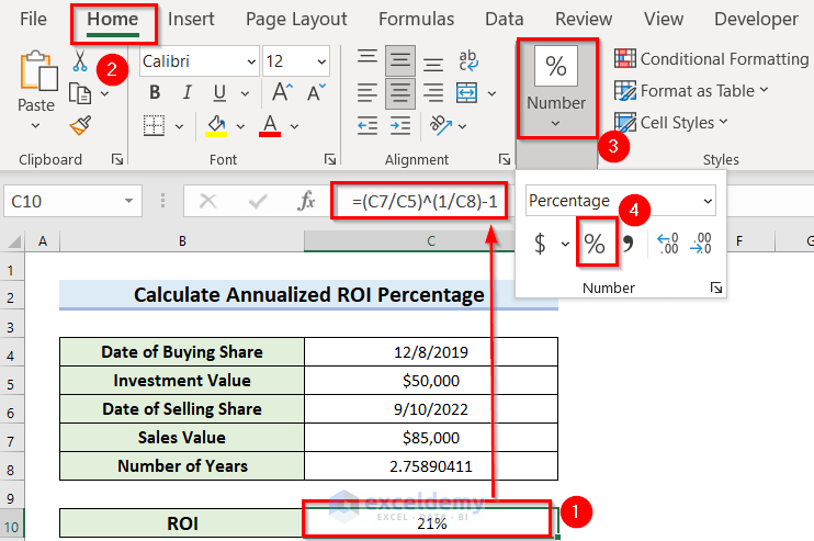
- Select C10 to calculate the ROI percentage.
- Use the formula in C10.
=(C7/C5)^(1/C8)-1C8 cell contains the Number of Years and C7, and C4 contain the Sales Value and Investment Value.
- Press ENTER.
- Convert the result into percentage using the Number format in the Home tab.
You will see the ROI percentage.
Method 5 – Using the RATE Function to Calculate the Annual ROI Percentage
Steps:
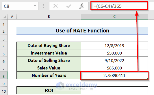
- Select C8 to keep the Number of Years.
- Use the formula in C8.
=(C6-C4)/365C6 cell contains the Date of Selling Share and C4 the Date of Buying Share. By subtracting the two dates you will get the total days in between. You must divide the result by 365 to find the Number of Years.
- Press ENTER.
You will get the Number of Years.
- Select C10 to see the ROI percentage.
- Use the formula in C10.
=RATE(C8,0,-C5,C7)- Press ENTER.
You will get the annual ROI percentage.
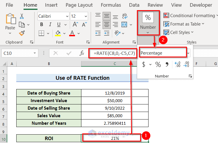
Formula Breakdown
The RATE function will return the annual rate of investment in percentage.
- C8 denotes the NPER as the share-holding period.
- 0 denotes that the annual payment is unknown.
- C5 denotes the Investment, and the Negative sign denotes that you have made the payment.
- C7 denotes the Sales value.
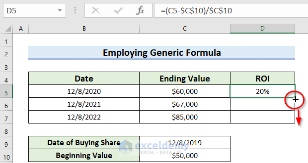
Method 6 – Estimating Each Year’s ROI Percentage in Excel
Steps:
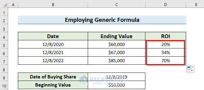
- Select D5:D7 to see the calculated ROI percentages.
- In the Home tab >> go to Number.
- Choose Percentage (%).
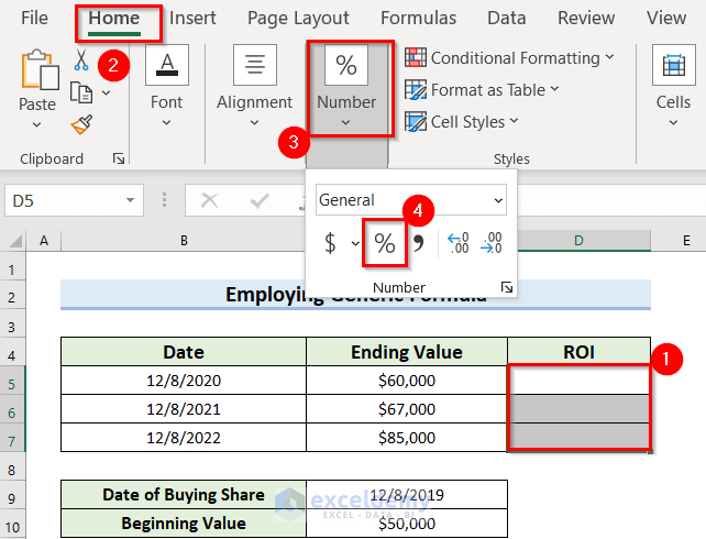
- Select D5 to calculate the ROI percentage.
- Use the formula in D5.
=(C5-$C$10)/$C$10C5 cell contains the Ending value and $C$10 contains the Beginning value. The Dollar sign ($) creates an absolute cell reference in C10.
- Press ENTER.
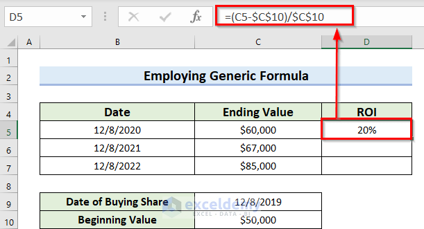
- Drag down the Fill Handle to see the result in the rest of the cells.
You will see the ROI percentages.
Read More: How to Calculate Expected Return in Excel
Tips to Calculate the ROI Percentage in Excel
You may need to increase or decrease the decimal places:
- Go to Number in the Home tab.
- Click Increase Decimal or Decrease Decimal.
Here, Increase Decimal was used. This is the output.

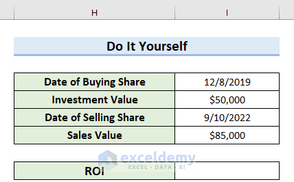
Practice Section
Practice here.
Download Practice Workbook
Download the practice workbook.
<< Go Back to ROI Calculation in Excel | Excel for Finance | Learn Excel
Get FREE Advanced Excel Exercises with Solutions!
