Latest Posts From Lutfor Rahman Shimanto

Make Schedule in Excel: Knowledge Hub Make a Daily Schedule in Excel Make an Hourly Schedule in Excel Create a Monthly Schedule in Excel Create a ...

Maximize Excel efficiency with shortcuts like Ctrl+C/V, freeze panes for scrolling, and use "Format as Table" for better data management. Master PivotTables, ...

Inventory Management in Excel: Knowledge Hub Maintain Store Inventory in Excel Keep Track of Inventory in Excel Make Inventory Aging Report in Excel ...

This tutorial will cover several methods in Excel for Time Conversion. We'll walk you through converting time into hours, minutes and seconds. You will also ...

Download Practice Workbook Organize Sheets.xlsm Example 1 - Apply Shortcuts to Highlight Sheet Select range B5:D9 >> press Alt+H+L+N. ...

Blank in Pivot Table: Knowledge Hub Show Zero Values in Excel Pivot Table Hide Zero Values in Excel Pivot Table Remove Blank Rows in Excel Pivot ...
Suppose you have the following dataset to use for a 3D Scatter Plot. Insert a Scatter Chart Steps: Select the active range (B4:D16 in this ...

Pivot Table Value Field Settings: Knowledge Hub Create a Pivot Table with Values as Text Calculate Median in Excel Pivot Table << Go ...
Here's an overview of converting coordinates into latitude and longitude. Download the Practice Workbook Easting Northing to Lat Long.xlsm ...

Pivot Table Date Format: Knowledge Hub Change Date Format in Pivot Table in Excel Remove Time from Date in Pivot Table << Go Back to ...

Cubic Spline Interpolation is a curve-fitting method to interpolate a smooth curve between discrete data points. We use this interpolation in various ...

One of the most helpful software you can use is Microsoft Excel. It is possible to do an endless number of things with a dataset by utilizing Excel's ...

This article will discuss two causes and solutions for why the Number Format might not be working. Number Format Is Not Working in Excel: 2 Reasons ...
The fundamental goal of inventory control is to guarantee that sufficient items or resources are available to fulfill demand without generating surplus ...

Microsoft Excel is a helpful program. You can conduct infinite operations on a dataset using Excel's tools and capabilities. Regularly, we must search for data ...
See Our Reviews at


Hello Raj
Thank you for reaching out with your comment. You encountered a different result than what was described in the post. I assume that you missed inserting positive numbers in the range C16:C17. However, once those values were included, I discovered a result identical to what is described in the post. Therefore, It’s essential to ensure all intended data is inputted correctly.
Regards
Lutfor Rahman Shimanto
Hello Charlotte Fahey
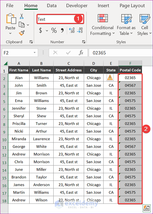
Thank you for reporting on this fascinating issue. I experience the same problems when a postal code begins with 0, and it is essential to preserve the leading zero when entering data into the system or application.
The Postal Code column must be formatted as text. Following that, insert the desired data.
Now, adhere to the methods mentioned in this article. Ideally, you will observe the desired results.
Regards
Lutfor Rahman Shimanto
Thank you for bringing this issue to my attention, William Wyatt. I understand that you have been experiencing difficulties using formulas on cells formatted as fractions in your workbook. I apologize for any confusion or frustration this may have caused you.
I have gone through this article and did not experience any of your issues. I am using Microsoft 365 to investigate this case. Could you share your workbook with us via email to better understand your situation? I would appreciate it if you could assist me more effectively.
Regards
Lutfor Rahman Shimanto
Hello DEBB WOLFE
We appreciate your comment. I understand your difficulty, and you can avoid the issue by importing the CVS file into the existing worksheet.
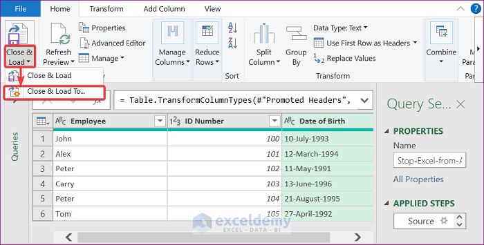
Change the column type in the Power Query window to text, as this article mentions. Next, select the Home tab. Select Close & Load and then Close & Load To at a later time.
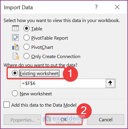
As a result, the Import Data window will display. Check the Existing Worksheet and then press OK.
Thus, you will be able to solve the problem.
Regards
Lutfor Rahman Shimanto
Hello ARON HOLMBERG
Thank you for reporting your issues. To count the number of components for each station, when the Station ID may be in one of three different columns, you can use the SUMPRODUCT function.
=SUMPRODUCT((InputSheet!$B:$B=B5)+(InputSheet!$C:$C=B5)+(InputSheet!$D:$D=B5))
This formula will test each of the three columns for the station ID and return 1 if it’s present in any of the columns and 0 if it’s not. Then, SUMPRODUCT will sum up the results, giving you the components for the station.
This solution is more elegant than creating a new column that combines the three columns, as it avoids the need to manipulate the data. If you would like a copy of the illustrated workbook, please click the link provided below this section.
https://www.exceldemy.com/wp-content/uploads/2023/01/To-Count-the-Number-of-Components-for-Each-Station.xlsx
Best regards,
Lutfor Rahman Shimanto
Hello ABIGAYLE PAULSON
Thank you for reporting on this fascinating issue. I have reviewed this article and found an interesting idea to solve your problem. For illustration, let’s walk through 2nd Example. Filtering the dataset (Sheet3) based on cell values on another sheet (Sheet4). The context filters the dataset for Apple or Tomato products.
VBA Code:
If the changed cell is either C2 or E2, the macro will execute and filter the data in “Sheet3” based on the new values in these cells. Note that the Worksheet_Change event must be placed in the code module for the “Sheet4” worksheet.
The changes we must make to the original code to create the auto-filtering behavior:
1) We have to add a Private Sub Worksheet_Change(ByVal Target As Range) procedure to the code module for the “Sheet4” worksheet. This procedure runs automatically whenever a cell value is changed on this worksheet.
2) We can add an If statement to check whether the changed cell is in Sheet4 and C2 or E2. If so, the macro continues executing; if not, it exits without doing anything.
3) We need to move the Dim statements for product1 and product2 inside the If statement, so they are only declared if the macro is going to run.
4) The rest of the macro code is the same as the original code, so it will apply the same filter to “Sheet3” based on the new values in “Sheet4” whenever the cell value changes.
By adding this Worksheet_Change procedure to the code module, the macro will run automatically whenever a change is made to the specified cells in “Sheet4” without manually opening and running the macro.
Regards
Lutfor Rahman Shimanto
Hello Chris
Thanks for your comment! You want to insert multiple leave records at a time.
I have reviewed your requirements. I am delighted to inform you that I have found an idea that uses an Excel UserForm to fulfil your goal. Please check the following:
To improve the Excel file, I had to write many lines of code and adjust many features, so I am not explaining how I did this. You can down the improved file from the following link: https://www.exceldemy.com/wp-content/uploads/2024/06/Chris-SOLVED.xlsm
Hopefully, you will like the idea. Good luck.
Regards
Lutfor Rahman Shimanto
Excel & VBA Developer
ExcelDemy
Hello Sherry
Thanks for reaching out! Providing an ultimate solution without glancing at your Excel file is difficult. However, I suggest several things you may check to ensure the multi-selection drop-down works properly.
Ensure you have created named ranges for your dataset as described. Make sure that the strDVList variable correctly references your named range. To ensure that the named range CityNames is correctly referenced by strDVList, you can call the InitializeDVList subroutine in the Worksheet_SelectionChange event before it tries to use strDVList.
So, double-click on the user form and replace the existing code with the following:
Hopefully, these ideas will help you overcome your situation. Good luck.
Regards
Lutfor Rahman Shimanto
Excel & VBA Developer
ExcelDemy
Hello Cathy Thompson
Thanks for visiting our blog! We cannot provide an ultimate solution without reviewing your Excel file and being remote. However, you apply several adjustments to the dataset, like checking for non-numeric characters, converting text to numbers, ensuring correct formatting, and checking calculation mode. To clean up your numeric data, you can create a helper numeric column (e.g., real estate tax) and use the formula:
=VALUE(TRIM(CLEAN(B1)))Lastly, sum the values in the helper columns using the SUM function.Hopefully, these ideas will help. If you still have difficulties, you can share your problem with the ExcelDemy Forum by attaching your Excel file. Good luck.
Regards
Lutfor Rahman Shimanto
ExcelDemy
Hello Onkar
Thanks for your invaluable feedback!
When copying data from the Excel files, you wanted a sub-procedure to copy only the header from the first file and skip the header row for the subsequent files. Currently, you are getting the runtime error 1004 with the existing code, which is typically caused by issues with object references or out-of-bound ranges.
Don’t worry! I have reviewed your problem and improved the existing sub-procedure to fulfil your goal. Please check the following:
Improved Excel VBA Sub-procedure:
Hopefully, with the code, you will not get any runtime error, and you will be able to copy the header only from the first filter, skipping the header row for the other files. I have attached the solution workbook used to solve your problem. You can download it for better understanding. Good luck.
DOWNLOAD SOLUTION WORKBOOK
Regards
Lutfor Rahman Shimanto
Excel & VBA Developer
ExcelDemy
Hello John
Thanks for your compliments! Your appreciation means a lot to us.
I have reviewed your requirements. To do so, first, you must create helper cells to store the dates associated with each checkbox when marked TRUE. Next, use the MAX function to find the latest date from these helper cells. Finally, the latest date calculates the new expiration date in A27. Please check the following:
Follow these steps:
Hopefully, these ideas will help you reach your goal. I have attached the solution workbook as well. Good luck.
DOWNLOAD SOLUTION WORKBOOK
Regards
Lutfor Rahman Shimanto
ExcelDemy
Hello Shaz
Thanks for your question! You want to link checkboxes directly to the same cells where these are presented.
To do so, insert a check box and edit the text like described here. Next, select the checkbox by holding the Ctrl key. Now, type the cell reference in the formula bar where the checkbox is located. Please check the following:
You can download the workbook used to solve your problem: https://www.exceldemy.com/wp-content/uploads/2024/06/Shaz-SOLVED.xlsx
Regards
Lutfor Rahman Shimanto
ExcelDemy
Hello David Wang
Thanks for your kind words! You are very welcome.
I have reviewed both of your requirements. These requirements can quickly be developed, and I think they will overcome all your hassles. I have made the necessary changes. Please check the following:
To fulfil your goal, I had to make many changes to the codes and design, develop several sub-procedures and event procedures, and add the necessary validation. As there are many more things, I am not describing everything here. If you are interested in how I developed such a customized date picker, you can post your queries in the ExcelDemy Forum.
Hopefully, you have found the solution you were looking for. I have attached the Date Picker file. Good luck.
DOWNLOAD CUSTOMIZED DATE PICKER
Regards
Lutfor Rahman Shimanto
Excel & VBA Developer
ExcelDemy
Hello Lisa Hoffer
Thanks for visiting our blog and sharing such an interesting question. You wanted an Excel VBA sub-procedure to clear the contents of non-contiguous rows. I have developed such a sub-procedure to fulfil your goal. Please check the following:
Excel VBA Sub-procedure:
Hopefully, you have found the VBA macro you were looking for. I have attached the workbook used to solve your problem. Good luck.
DOWNLOAD SOLUTION WORKBOOK
Regards
Lutfor Rahman Shimanto
Excel & VBA Developer
ExcelDemy
Hello Robert
Thanks for your question! You want to calculate the number of weeks between two dates. To do so, you can apply several formulas:
Hopefully, you have found the solutions you were looking for. I have attached the solution workbook as well. Good luck.
DOWNLOAD SOLUTION WORKBOOK
Regards
Lutfor Rahman Shimanto
ExcelDemy
Dear Jess
Thanks for your comment! Only leading spaces typically don’t affect the SUM function in most Excel versions. However, leading spaces can indeed cause numbers to be treated as text in some Excel versions like yours. It is great to hear that removing leading spaces resolved the issue for you.
I am sharing another exciting solution for summing numbers with inconsistent spaces using an Excel formula. Please check the following:
Excel Formulas (using SUM, VALUE, and SUBSTITUTE functions):
=SUM(VALUE(SUBSTITUTE($B$2:$B$7, " ", "")))Hopefully, you will like the solution. Good luck.
Regards
Lutfor Rahman Shimanto
ExcelDemy
Hello Michael A. Dunn
Thanks for visiting our blog and noticing a critical fact. You were right. Sorry for the inconvenience. We have improved all the formulas and modified the article.
Using the arithmetic formula would be best if you worked with a fixed rate. So, it may provide different results from other procedures. However, all the procedures except for using the arithmetic formula will calculate almost the same result. So, if you do not have a fixed rate, consider applying the formulas Using Nested IF, IFS and SUMPRODUCT functions.
Regards
ExcelDemy
Dear Doug
Thanks for visiting our blog and sharing an exciting problem. You needed help with some Excel VBA sub-procedures to move rows from the Account sheet to the Archive sheet under specific conditions. You want this to happen only when you click a button on the Metrics sheet and turn it on. The conditions are as follows: if a row in the Account sheet has Closed or Archive in its Status column. You also wanted a pop-up to confirm the action before moving a row. Additionally, the row should be deleted from the Account sheet after moving.
Don’t worry! I have reviewed your requirements and demonstrated the situation within an Excel file with a suitable dataset. I have solved the problem with the help of some Excel VBA sub-procedures. Please check the following:
Excel VBA Sub-procedures:
Hopefully, you have found the solution you were looking for. I have attached the solution workbook as well. Good luck.
DOWNLOAD SOLUTION WORKBOOK
Regards
Lutfor Rahman Shimanto
Excel & VBA Developer
ExcelDemy
Hello there! Thanks for sharing an exciting problem. Since using the conditional formatting option for text alignment is impossible, you can only use an Excel VBA procedure.
Note: The event procedure will trigger when range B2:B7 is changed. If the cell value is Red, it will apply left alignment. For Blue, it will be center alignment; for the other values, it will apply left alignment. You can modify the code based on your needs.
Excel VBA Event Procedure:
Hopefully, the solution will fulfil your goal. Download the attached solution workbook for a better understanding.
DOWNLOAD SOLUTION WORKBOOK
Regards
Lutfor Rahman Shimanto
Excel & VBA Developer
ExcelDemy
Dear, Thanks for pointing out the fact! You are right. The Alignment tab in the Format Cells dialog box is unavailable when setting up conditional formatting rules. So, using the conditional formatting option for text alignment is impossible.
Don’t worry! There is an idea of using an Excel VBA event procedure. Please check the following:
The event procedure will trigger when range B2:B7 is changed. If the cell value is Red, it will apply left alignment. For Blue, it will be center alignment; for the other values, it will apply left alignment.
Excel VBA Event Procedure:
Hopefully, the solution will fulfil your goal. I have attached the solution workbook as well. Good luck.
DOWNLOAD SOLUTION WORKBOOK
Regards
Lutfor Rahman Shimanto
Excel & VBA Developer
ExcelDemy
Dear, Thanks for your compliment! That’s fantastic to hear! We are glad the template was helpful. Keeping track of sales data can be overwhelming, but a well-designed sales tracker can make a difference.
Regards
ExcelDemy
Dear Naqavi
Thanks for your compliment! Your appreciation means a lot to us.
Regards
ExcelDemy
Hello Umar
Thanks for visiting our blog and sharing an exciting problem. You want to apply Data validation in two columns, with options in the second column dependent on the first column selection.
Don’t worry! I have demonstrated your situation within an Excel file and solved it. Please check the following:
You can download the solution workbook for a better understanding: https://www.exceldemy.com/wp-content/uploads/2024/06/Umar-SOLVED.xlsx
Regards
Lutfor Rahman Shimanto
ExcelDemy
Dear Annie
Thanks for visiting our blog and sharing an important fact! You are right that the holiday range reference shifts when you copy the formula. You need to use absolute references for the holiday range to fix the issue. Another improvement you can consider is not keeping the holiday list and start date or next working dates in the same column. Assume the start date and next working date data are in columns B and C; the holiday list is in column E.
Don’t worry! I have demonstrated an improved Excel file to overcome the situation. Please check the following:
Follow these steps:
Hopefully, you have found the solution you were looking for. I have attached the solution workbook as well. Good luck.
DOWNLOAD SOLUTION WORKBOOK
Regards
Lutfor Rahman Shimanto
ExcelDemy
Hello Brandy
Thanks for your wonderful compliment! Your appreciation means a lot to us.
The Error 13 Type Mismatch in VBA typically occurs when you try to perform an operation on incompatible data types. I have reviewed the code and found that Value2 is used to contain cell values when looping through and comparing with Value1. It seems like some of your values contain errors, which is why it is not possible to use the Len function with this value. So, to avoid this type of situation, you can use IsError to check whether the cells contain any errors or not. If not, perform an operation; otherwise, do nothing.
You can use the following structure:
Hopefully, you have found the ideas you were looking for. Good luck.
Regards
Lutfor Rahman Shimanto
Excel & VBA Developer
ExcelDemy
Hello Mary
Thanks for visiting our blog and sharing your problem. The issue you are facing is due to the RAND function, which generates a new random number every time the worksheet recalculates.
To prevent the problem, copy the random values, then use Paste Special and paste them back as Values. The idea should keep your random names stable.
Regards
ExcelDemy
Dear, Thanks for your question! Unfortunately, it isn’t possible to disable copying directly within Excel Online. Excel Online offers some control over how users interact with a shared workbook, but it doesn’t provide a direct way to turn off copying explicitly. You can set the workbook to Read Only for users who cannot copy data.
Regards
Lutfor Rahman Shimanto
ExcelDemy
Hello Luke
Thanks for sharing your problem with such clarity. Based on your requirements, you can use the following Excel VBA Sub-procedure to fulfil your goal.
Excel VBA Sub-procedure:
Hopefully, the sub-procedure will be helpful. Stay blessed.
Regards
Lutfor Rahman Shimanto
Excel & VBA Developer
ExcelDemy
Hello Luke
Thanks for reaching out and sharing an exciting problem.
You want to generate a comma-delimited (.txt) file from an Excel sheet. When saving as CSV, you want to remove the double quotes that Excel automatically adds. The text file should have each data point separated by commas, without any quotes surrounding the text.
Don’t worry! I have developed an Excel VBA code to help you overcome your situation. Please check the following:
Excel VBA Sub-procedure:
I hope you have found the solution you were looking for. I have attached the solution workbook. Good luck.
DOWNLOAD SOLUTION WORKBOOK
Regards
Lutfor Rahman Shimanto
Excel & VBA Developer
ExcelDemy
Hello Nancy Cruz
Thanks for visiting our blog! And also sharing your problem with such clarity. I have reviewed your issue with date formatting and come up with a solution. Please check the following:
Follow these steps:
mm/ddHopefully, you have found the solution you were looking for. I have attached the solution workbook as well. Good luck.
DOWNLOAD SOLUTION WORKBOOK
Regards
Lutfor Rahman Shimanto
ExcelDemy
Hello Pablo
Thanks for visiting our blog and sharing your queries! You can modify the existing code slightly to update specific columns or rows in Google Sheets from Excel. Follow the previously mentioned steps, ensure you have the necessary permissions for the Google Sheet and adjust these with the VBA code.
Excel VBA Code:
Things to keep in mind: To adjust the VBA code, replace YOUR_SPREADSHEET_ID with your actual Google Sheet ID, and replace your YOUR_CLIENT_ID and YOUR_CLIENT_SECRET with the values from your OAuth 2.0 credential JSON file. Adjust the rangeName to specify the exact range (column/row) you want to update in the Google Sheet. Next, modify dataToUpdate to include the data you want to update. After running the VBA code, it will open a browser for you to authenticate with Google; enter the authorization code.
Hopefully, the code will fulfil your goal. Good luck.
Regards
Lutfor Rahman Shimanto
Excel & VBA Developer
ExcelDemy
Hello Rahul Dixit
Thanks for visiting our blog and sharing such an exciting problem! I have reviewed your problem and come up with an Excel VBA User-defined function. Please check the following:
Excel VBA Code:
Hopefully, you have found the solution you were looking for. I have attached the solution workbook as well; good luck.
DOWNLOAD SOLUTION WORKBOOK
Regards
Lutfor Rahman Shimanto
Excel & VBA Developer
ExcelDemy
Hello, Rekayasa Perangkat Lunak Aplikasi!
Thank you for your question. The main purpose of the Excel sales template provided in the article is to facilitate the recording and analysis of sales data for any merchandising business. Also, this comprehensive template includes various sections, such as a sales summary, a sales recording table, sales performance analyses, and a sales plan template. It helps businesses track sales transactions, compare planned versus actual sales, and analyze overall sales performance, enabling more informed decision-making and strategic planning.
If you have any further questions about the article or the templates, feel free to ask!
Regards
ExcelDemy
Dear Jon Peltier
Thanks for your invaluable feedback and suggestions! You are correct about the positive percentage error bars being inserted incorrectly. Based on your suggestions, we have updated the article section.
Regards
ExcelDemy
Hello Parvez Alam
Thanks for the compliment! You can include the “RefreshAll” command to refresh all Power Query connections. Don’t worry! I have improved the code a bit to fulfil your goal.
Excel VBA Code:
I hope you have found the code you were looking for. Good luck.
Regards
Lutfor Rahman Shimanto
Excel & VBA Developer
ExcelDemy
Hello Vickie
Thanks for visiting our blog and sharing an exciting problem with such clarity. I have reviewed your situation and developed two sub-procedures to fulfil your goal. Your problem is about automating email alerts in Excel based on conditional formatting for expiry dates of lifting equipment test certificates.
Don’t worry! I have demonstrated it in an Excel workbook. Please check the following:
Excel VBA Sub-procedure:
I hope you have found the sub-procedures you were looking for. I have attached the solution workbook as well. Good luck.
DOWNLOAD SOLUTION WORKBOOK
Regards
Lutfor Rahman Shimanto
Excel & VBA Developer
ExcelDemy
Hello Mohammed
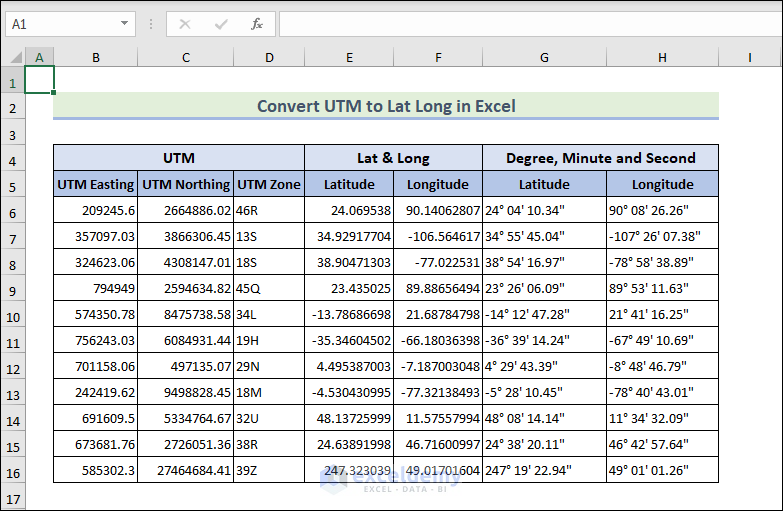
Thanks for sharing your problem! However, we can not accurately get the corresponding latitude and longitude values using only the UTM Easting and UTM Northing. We also need UTM Zone, Easting, and Northing values to get Lat and Long values.
For your address, the UTM Zone would be 39Z. Let’s say your UTM Easting, UTM Northing, and UTM Zone are 585302.3, 27464684.41, and 39Z. Using this UTM information, you can get the corresponding Latitude and Longitude. To achieve your goal, I have developed some Excel VBA User-defined functions.
Follow these steps:
Hopefully, these user-defined functions will help. I have attached the solution workbook as well.
DOWNLOAD SOLUTION WORKBOOK
Regards
Lutfor Rahman Shimanto
Excel & VBA Developer
ExcelDemy
Hello David
Thanks for visiting our blog! For your address, the UTM Zone would be 32U. Let’s say your UTM Easting, UTM Northing, and UTM Zone are 691609.5, 5334764.67, and 32U. Using this UTM information, you can get the corresponding Latitude and Longitude. To achieve your goal, I have developed some Excel VBA User-defined functions.
Follow these steps:
Hopefully, these user-defined functions will help you reach your goal. I have attached the solution workbook as well. Good luck.
DOWNLOAD SOLUTION WORKBOOK
Regards
Lutfor Rahman Shimanto
Excel & VBA Developer
ExcelDemy
Dear Sanjeev
Thanks for visiting our blog and sharing your problem. After adding the desired rows, you must drag the Fill Handle icon to copy the existing formulas for new employees. We have improved the file and made the necessary formula adjustments based on your goal.
SOLUTION Overview:
You can download the solution file: https://www.exceldemy.com/wp-content/uploads/2024/05/Sanjeev-Fernandes-SOLVED.xlsx
Regards
Lutfor Rahman Shimanto
ExcelDemy
Dear Jen
Thanks for explaining your requirements clearly. I have reviewed the existing user-defined function and tried to improve it to achieve your goal. The improved user-defined function will try to populate house numbers, roads, cities, states and zip codes by taking Lat and Long values; if any item is missing, it will display an extension like Incomplete!
Follow these steps:
I hope you have found the user-defined function of reverse geocoding you were looking for. I have attached the solution workbook as well. Good luck.
DOWNLOAD SOLUTION WORKBOOK
Regards
Lutfor Rahman Shimanto
Excel & VBA Developer
ExcelDemy
Hello Watt
Thanks for visiting our blog and sharing your queries. I have reviewed your requirements. Unfortunately, you cannot directly use any formulas to add a hidden apostrophe. Formulas can only output visible characters; not even a User-defined function can do that. So, you can type the apostrophe before the number or text to do so, though it is very exhausting when it comes to lots of cells.
Don’t worry! I have developed a sub-procedure that will add a hidden apostrophe to cells in a selected range without displaying it with one click.
SOLUTION Overview:
Excel VBA Sub-procedure:
Hopefully, you will find the solution helpful. I have attached the solution workbook as well; good luck.
DOWNLOAD SOLUTION WORKBOOK
Regards
Lutfor Rahman Shimanto
Excel & VBA Developer
ExcelDemy
Dear Iona
Thanks for visiting our blog and sharing your requirements! I have reviewed your goal and created an Excel VBA Event procedure (assuming your dates are in column A).
Excel VBA Event Procedure:
Right-click on the sheet name tab, paste the given code into the sheet module and save it. Hopefully, the idea will fulfil your goal; good luck.
Regards
Lutfor Rahman Shimanto
Excel & VBA Developer
ExcelDemy
Hello James
Thanks for your compliment! We are glad these ideas helped you a lot.
You are facing difficulties in excluding blank cells that hold a formula from the print area. The following code can give you ideas; here, the HasFormula property is used, along with checking whether it is empty or not.
Excel VBA Code:
I hope the ideas will help you exclude blank cells holding a formula. Good luck.
Regards
Lutfor Rahman Shimanto
Excel & VBA Developer
ExcelDemy
Dear Abinsh
Thanks for sharing your requirements. You want to convert numbers to words in Qatar Riyal. Don’t worry! I have modified the previously given code to fulfil your goal.
Excel VBA User-Defined Function:
I hope you have found the solution you were looking for. I have attached the solution workbook. Good luck.
DOWNLOAD SOLUTION WORKBOOK
Regards
Lutfor Rahman Shimanto
Excel & VBA Developer
ExcelDemy
Hi Diw
Thanks for thanking me! All three ideas clear the Excel memory cache. However, they differ in the approaches and memory they target.
So, it would be better to clear PivotCache Memory for heavy workbooks. You can apply Nothing Literal to any unwanted object for general memory cleanup. For a slight memory boost, you can assign zero to RecentFile Properties.
I hope these ideas will help you. Thanks once again for visiting our blog. And good luck.
Regards
Lutfor Rahman Shimanto
ExcelDemy
Hello Fazlay Rabby
Thanks for your compliment! You are very welcome. We are glad that you found the article helpful.
Regards
Lutfor Rahman Shimanto
ExcelDemy
Hello Barry
Thanks for your compliment. Your appreciation means a lot to us. Thanks once again for sharing an exciting problem.
I have reviewed your requirements. You wanted to place small rectangles at each of the 12 positions on a clock face. Besides, each shape will be placed at an angle of 30 degrees; more than its neighbor. Don’t worry! I have come up with a sub-procedure and a user-defined function to fulfill your goal.
SOLUTION Overview:
Excel VBA Sub-procedure:
I hope you have found the solution, you were looking for. I have attached the solution workbook as well; good luck.
DOWNLOAD SOLUTION WORKBOOK
Regards
Lutfor Rahman Shimanto
Excel & VBA Developer
ExcelDemy
Hi Nat
Thanks for your patience and feedback. We apologize for any confusion. While the article covers two common reasons for date filter issues, other factors might be at play in your case.
You mentioned trying the two solutions and not getting the desired results. We recommend joining our ExcelDemy Forum. You can post your question there and attach your Excel file for a more detailed look.
Regards
Lutfor Rahman Shimanto
ExcelDemy
Dear Harman
Thanks for thanking me. You are most welcome. We are glad the solution worked perfectly.
Regards
ExcelDemy
Hello Fulad
Thanks for your compliment! As you requested, you can use the following dataset, which contains data with your mentioned fields:
You can download the workbook from the following link:
DOWNLOAD WORKBOOK
I hope you have found the dataset you were looking for; good luck.
Regards
Lutfor Rahman Shimanto
ExcelDemy
Hello Olaide
Thanks for thanks! You are very welcome. Your appreciation means a lot to us.
You are right! The user-defined function works perfectly fine for a few sets of coordinates. I have reviewed the code and estimated the time required to perform it on a pair of coordinates; it takes 5.7 seconds on my machine (the time can vary from device). It will take almost 8 hours to perform 5000 sets of coordinates with a spontaneous internet connection.
The user-defined function mentioned in this article uses the OpenStreetMap Nominatim API to perform reverse geocoding. It retrieves location information based on the lat and long values given to it. It must take the required time to perform perfectly.
So, it is impossible to reverse geocode 5000 sets of coordinates within minutes. If you ever feel like getting location information without applying the user-defined function like the regular Excel function, you can use the following sub-procedure. You need to run the code, and it will consider the lat and long values as columns B and C starting from row 3 and display the result in column D.
I hope you understand the situation. Stay blessed.
Regards
Lutfor Rahman Shimanto
Excel & VBA Developer
ExcelDemy
Hello Alan Ang
Thanks for visiting our blog and asking an interesting question. You seek the language codes for Simplified Chinese, Traditional Chinese, and Central Khmer. Please check the following table:
You can easily translate and fulfil your goal using the above language codes and the user-defined function mentioned in this article.
I hope you have found the language code you were looking for. I have attached the workbook used to investigate your question; good luck.
DOWNLOAD WORKBOOK
Regards
Lutfor Rahman Shimanto
ExcelDemy
Dear, Thanks for visiting our blog and sharing your questions. You want to modify the existing formula to deal with the southerly direction of the bearings. The provided formulas in the article work for any bearing, regardless of direction. This is because the SIN and COS functions account for the direction within their calculations.
Southerly bearings typically range from 180 to 270 degrees. The formulas will handle these values fine and automatically calculate the appropriate change in Northing and Easting based on the southerly direction. The cosine value for bearings in this range will be negative, meaning there will be a decrease in Northing because the reference point is likely north of the new point. Likewise, the sine value will be positive, meaning an increase in Easting because a southerly direction moves the point eastward.
So, you don’t need to modify the formulas for southerly directions. They will work as intended.
Regards
Lutfor Rahman Shimanto
ExcelDemy
Dear Adam
Thanks for your feedback. I have reviewed your requirements. It seems like you want to perform a lookup of multiple entries (country names) in a single cell separated by a delimiter, such as commas. There will be a lookup table to keep the corresponding short names for each country. You are looking for a complex formula that takes multiple country names separated by commas, returns corresponding values (country short names), and displays them in a single cell.
Don’t worry! I have demonstrated your situation and developed a complex formula to fulfil your goal. I used the TEXTJOIN, INDEX, MATCH, TRIM, and TEXTSPLIT functions to build the formula.
SOLUTION Overview:
Suppose you want to enter the comma-separated country names in cell E1. In cell E2, you want to display country short names. To do so,
I hope you have found the formula you were looking for. I have attached the solution workbook as well; good luck.
DOWNLOAD SOLUTION WORKBOOK
Regards
Lutfor Rahman Shimanto
ExcelDemy
Hello Harman
Thanks for visiting our blog and sharing your query. You want 0 as leading when returning a number against a character. Don’t worry! I have come up with two solutions:
Use of TEXTJOIN, TEXT & VLOOKUP Functions
Use of VBA User-Defined Function
I hope the formulas and VBA code will fulfil your goal. I have attached the solution workbook; good luck.
DOWNLOAD SOLUTION WORKBOOK
Regards
Lutfor Rahman Shimanto
Excel & VBA Developer
ExcelDemy
Hello Anon
Thanks for your question! You wanted formulas to check for changes in multiple columns. Assuming you have three columns: First Name, Middle Name, and Last Name, you want to check for changes in the Timestamp column.
Solution Overview:
Follow these steps:
Now, input the intended names to see the output, like the GIF above.
I hope these are the formulas you were looking for. I have attached the solution workbook; good luck.
DOWNLOAD SOLUTION WORKBOOK
Regards
Lutfor Rahman Shimanto
ExcelDemy
Hello Charlie V
Thanks for visiting our blog and sharing your ideas. You are talking about shortcut keys to hide all rows or columns.
Do worry! We have demonstrated the whole idea. Please check the following GIF:
Required Shortcut Keys to Hide All Rows or Columns:
>> Ctrl + Shift + Right Arrow to select all columns to the right.
>> Ctrl + 0 to hide the selected columns.
>> Ctrl + Shift + Down Arrow to select all rows to the bottom.
>> Ctrl + 9 to hide the selected rows.
Hopefully, these are the shortcut keys you were looking for. Once again, thanks for the comment; good luck.
Regards
Lutfor Rahman Shimanto
ExcelDemy
Hello Steve Zimmermann
Thanks for visiting our blog and sharing your problem. You mentioned that the existing article methods work fine for regular Excel but not when opened inside SolidWorks (SW). Instead of showing the cell color, you get a #BLOCKED! Error; it shows up when a required resource can not be accessible.
It seems there are compatibility issues between VBA functionalities and SolidWorks. When Excel is opened by other applications like SolidWorks, some features and functionalities may not be available. As a result, when some resources are unavailable, they show #BLOCKED!
To overcome your situation, you can check the settings related to external scripting. You can also reach out to the SolidWorks community forum. Providing a solution without glancing at your file and being remote is very tough. I hope these ideas will help you; good luck.
Regards
Lutfor Rahman Shimanto
ExcelDemy
Hello Abdul
Thanks for visiting our blog and sharing your requirements. You wanted to calculate the number of hours worked by each employee in a month. You also mentioned that you have 4 guards, 2 on day and 2 on night shifts. If each shift is 6 hours long and there are 4 shifts in a day, you can calculate the total hours worked by multiplying 6 by the total shits.
You have demonstrated your situation within an Excel file. You can download it by clicking the following link.
DOWNLOAD SOLUTION WORKBOOK
Note: If you want to display more detailed information like calculating exact amount of work time, you must create columns for start and end times. Then, calculate the hours worked for each shift by subtracting the start time from the end time.
I hope these ideas will help you overcome your problem; good luck.
Regards
Lutfor Rahman Shimanto
ExcelDemy
Dear Peter Berger
Thanks for your feedback. Perhaps you are right about using the direct results from Nominatim, which would lead to more accurate outcomes. However, we have to get the result from the response from the Nominatim API.
In addition to your previous post, you wanted to get all the information in a column but in different cells. Do not worry! I have improved the previously given code by using a 2D array.
SOLUTION Overview:
Required Excel VBA User-Defined Functions:
Hopefully, you have found the idea helpful. Download the solution workbook. Stay blessed.
DOWNLOAD SOLUTION WORKBOOK
Regards
Lutfor Rahman Shimanto
Excel & VBA Developer
ExcelDemy
Hello Peter Berger
Thanks for your nice words. Your appreciation means a lot to us.
You wanted to get all the address information in different columns. To do so, I have developed another assistive VBA user-defined function and improved the existing user-defined function named ReverseGeocoder. Using these two functions, you can quickly fulfil your goal.
Follow these steps:
I hope you have found the VBA user-defined function helpful. I have attached the solution workbook; good luck.
DOWNLOAD SOLUTION WORKBOOK
Regards
Lutfor Rahman Shimanto
Excel & VBA Developer
ExcelDemy
Hello James Martin
Thanks for visiting our blog and sharing your problem. When working with this code in another workbook, you are facing “Compile error: User-defined type not defined“. This error typically occurs when the required library or reference is not activated in the VBA Editor.
Initial Problem:
To overcome the problem, you must refer to the Microsoft VBScript Regular Expressions 5.5 library in VBA Editor.
SOLUTION Overview:
Press Alt+F11 >> Tools >> References >> Microsoft VBScript Regular Expressions 5.5 >> OK.
I have improved the codes and solved your problem in a workbook. You can find these codes in the modules. Hopefully, you have found the solution helpful. I have attached the solution workbook as well; good luck.
DOWNLOAD SOLUTION WORKBOOK
Regards
Lutfor Rahman Shimanto
Excel & VBA Developer
ExcelDemy
Dear Vyshnav V S
It is good to see you again. Thanks for sharing further requirements. You want to improve the existing VBA code to add a hyperlink in the email content. The hyperlink should display only the task ID, but when clicked, it will direct to the ALM link along with the task ID.
I have improved the previously given code to fulfil your goal. When sending an email, ensure that you uncomment the line that contains the “.Send” property. Also, change the existing base AML link with the intended one.
SOLUTION Overview:
Improved Excel VBA Sub-procedure:
I hope the improved sub-procedure will reach your goal. I have attached the solution workbook; good luck.
DOWNLOAD SOLUTION WORKBOOK
Regards
Lutfor Rahman Shimanto
Excel & VBA Developer
ExcelDemy
Hello Adele
Thanks for your nice words. We are glad you found the article helpful!
In Excel, we are directly unable to undo a VBA macro action in the same way you can undo regular actions using the Ctrl + Z shortcut. So, you must use the Excel Track Changes feature, or you can also use external version control systems like Git.
I hope these ideas will overcome your situation; good luck.
Regards
Lutfor Rahman Shimanto
ExcelDemy
Hello Harry Ingram
Thanks for such an interesting comment. You wanted to extract numbers even if there are decimal points. Additionally, if there are more numbers, you want to put them in different columns. I have come up with a solution using several Excel VBA User-defined functions.
SOLUTION Overview:
To do so, follow these steps:
I have also attached the solution workbook; good luck.
DOWNLOAD SOLUTION WORKBOOK
Regards
Lutfor Rahman Shimanto
Excel & VBA Developer
ExcelDemy
Hello Vyshnav V S
It is good to see you again. When sending a reminder email, you want to add a user interface instead of running the Excel VBA Sub-procedure. To achieve this goal, you must use an Excel UserForm. I have designed a user interface in an Excel File.
SOLUTION Overview:
I hope the solution will help you reach your goal. I have also attached the solution workbook; good luck.
DOWNLOAD SOLUTION WORKBOOK
Regards
Lutfor Rahman Shimanto
Excel & VBA Developer
ExcelDemy
Dear Vito Casalinuovo
Thanks for further clarifying your problem. Based on the requirement, I have come up with another solution, though the previous solution works perfectly on our end.
Assuming you have a dataset like the following:
You want to get all the tasks that fall on the same day. To achieve the goal, you can combine:
I hope these formulas will help you to reach your goal. I have attached the solution workbook as well; good luck.
DOWNLOAD SOLUTION WORKBOOK
Regards
Lutfor Rahman Shimanto
ExcelDemy
Hello Greg
Thanks for visiting our blog and informing us that the previous solution worked perfectly. You want to filter the data that includes the date falling within the specified date range (0 to 14 days). Also, you want to include the rows where the document submittal date is blank.
I have come up with an Excel VBA code. You can try it; if needed, make changes to fulfil your goal.
SOLUTION Overview:
Excel VBA Code:
I have attached the solution workbook; good luck.
DOWNLOAD SOLUTION WORKBOOK
Regards
Lutfor Rahman Shimanto
Excel & VBA Developer
ExcelDemy
Dear Vito Casalinuovo
It is good to see you again. Yes! You can capture all the tasks that fall on the same day. To do so, use the IFERROR, TEXTJOIN and FILTER function:
SOLUTION Overview:
Follow these steps:
I hope you have found the formula helpful. I am also attaching the solution workbook; good luck.
DOWNLOAD SOLUTION WORKBOOK
Regards
Lutfor Rahman Shimanto
ExcelDemy
Dear Vyshnav V S
It is good to see you again. You want to upgrade the previously given VBA code to include a feature that retrieves task details from an ALM system or a similar work item system.
To do so, connect to the ALM or work item system to fetch task details within the VBA. Later, you can develop a function to find the task details based on the task ID from the Excel sheet and generate a link to the task’s details. The implementation will depend on the system used and its access methods (like APIs).
Hopefully, the idea will help you; good luck.
Regards
Lutfor Rahman Shimanto
ExcelDemy
Dear Peter Summers
Thanks for visiting our blog and sharing your problem. You wanted to return a time value with “hh:mm”. To do so, you have to enhance your formula with the help of the TEXT function:
Hopefully, you have found the idea helpful; good luck.
Regards
Lutfor Rahman Shimanto
ExcelDemy
Dear Vyshnav V S
It is great to see you again. Thanks for reaching out and sharing another exciting problem.
To add a Request for Delivery Receipt and a Read Receipt in the Outlook Application, we must use the ReadReceiptRequested and OriginatorDeliveryReportRequested properties. Do not worry! Based on your new requirements, I have enhanced the existing sub-procedure (I provided earlier).
SOLUTION Overview:
Excel VBA SUb-procedure:
I hope you have found the solution you were looking for. The solution workbook is attached; good luck.
DOWNLOAD SOLUTION WORKBOOK
Regards
Lutfor Rahman Shimanto
Excel & VBA Developer
ExcelDemy
Hello Denny Hevalahu
Thanks for visiting our blog and sharing your questions.
To calculate the number of different individual items sold:
Hopefully, the formula will be helpful; good luck.
Regards
Lutfor Rahman Shimanto
ExcelDemy
Hello MEDO
Thanks for letting us know that the solution works perfectly on your end. However, you want to handle cultural settings in VBA, which also works on non-UK clients.
Assuming your requirements are related to the decimal separator and thousand separator settings. Different regions worldwide use different conventions to represent decimals and thousands of separators.
You can use two user-defined functions to replace these separators with periods and commas to overcome the situation. I have developed two VBA user-defined functions and slightly changed the existing sub-procedures.
Calculating Distance in Miles:
Calculating Distance in KM:
Hopefully, the VBA code will help you with your problem; good luck.
Regards
Lutfor Rahman Shimanto
Excel & VBA Developer
ExcelDemy
Hello Vito Casa
Thanks for visiting our blog and sharing your questions. Sheet1 contains a list of tasks with corresponding dates. You want to extract this information and plan the tasks on Sheet2 based on the dates. To do so, you can develop multiple formulas using VLOOKUP, INDEX, MATCH, and XLOOKUP. You can also use IFERROR to handle errors.
SOLUTION Overview:
NOTE: If you are a Microsoft 365 user, you will be able to use the XLOOKUP function.
I hope the formulas mentioned will reach your goal. I have attached the solution workbook as well; good luck.
DOWNLOAD SOLUTION WORKBOOK
Regards
Lutfor Rahman Shimanto
ExcelDemy
Dear Isaac Chavez
Thanks for visiting our blog. As requested, I have developed an Excel VBA Sub-procedure that will send an Email notification if the Deadline is 7 days ahead.
SOLUTION Overview:
Note: If the Microsoft Outlook dialog box appears, click Allow to send an email.
Excel VBA Sub-procedure:
I hope the sub-procedure will fulfil your requirements. I have attached the solution workbook as well; good luck.
DOWNLOAD SOLUTION WORKBOOK
Regards
Lutfor Rahman Shimanto
Excel & VBA Developer
ExcelDemy
Dear Vyshnav V S
As requested, I have improved the existing sub-procedure (previously provided) to fulfil your new requirements.
SOLUTION Overview:
NOTE: If the Microsoft Outlook dialog box appears, click Allow to send an email.
Improved Excel VBA Sub-procedure:
I hope the sub-procedure will reach your goal. I have attached the solution workbook as well; good luck.
DOWNLOAD SOLUTION WORKBOOK
Regards
Lutfor Rahman Shimanto
Excel & VBA Developer
ExcelDemy
Dear Vyshnav V S
Thanks for clarifying your requirements further. I have modified the previously given code to fulfil your goal. Now, you can select any column containing email IDs, and all the other required information will be retrieved from columns C and D.
SOLUTION Overview:
Excel VBA Sub-procedure:
Make changes to the code if necessary. I hope the code will fulfil your goal; good luck.
Regards
Lutfor Rahman Shimanto
Excel & VBA Developer
ExcelDemy
Dear Issac
Thanks for letting us know that the previously provided SendEmails sub-procedure worked on your side. Now, you want to automate this task daily. To achieve this, you create a Workbook_Open event and call the SendEmails sub-procedure. Later, you must use the Task Scheduler to open the workbook daily at a particular time. I have improved the SendEmails sub-procedure and created a solution to your problem using the mentioned idea.
Follow these steps:
Hopefully, you have found the ultimate solution to your requirements. I have attached the solution workbook; good luck.
DOWNLOAD SOLUTION WORKBOOK
Regards
Lutfor Rahman Shimanto
Excel & VBA Developer
ExcelDemy
Hello Vyshnav V S
Thanks for visiting our blog and sharing an exciting problem. I have developed an Excel VBA Sub-procedure that meets both requirements.
To send email using VBA, you can use the Send property. When sending an email, the Microsoft Outlook dialog box will appear. Lastly, you must click on Allow to send email.
SOLUTION Overview:
NOTE: Additionally, the sub-procedure will validate your selection. If you select another column instead of the ID column (assuming it is column B), the message will pop up saying to choose the intended column.
Excel VBA Sub-procedure:
Hopefully, the sub-procedure will meet your expectations. I have attached the solution workbook as well. Good luck.
DOWNLOAD SOLUTION WORKBOOK
Regards
Lutfor Rahman Shimanto
Excel & VBA Developer
ExcelDemy
Hello Irish Jim
Thanks for your compliments. Your appreciation and suggestions mean a lot to us. You are right; it would be great to mention right-clicking and clicking on View Code when inserting code in the sheet module. Also, it is important to mention the Target parameter when discussing events in Excel.
Thank you once again for visiting our blog and providing beneficial suggestions. Based on your suggestion, we have updated the sections. Hopefully, other visitors will have a better reading experience.
Regards
ExcelDemy
Hello Isaac Chavez
Thanks for visiting our blog and sharing your problem. I have developed an Excel VBA Sub-procedure that automatically sends emails.
SOLUTION Overview:
All you need to do is to click on Allow when the Microsoft Outlook dialog box appears.
Excel VBA Sub-procedure:
When testing the sub-procedure, I accidentally emailed you by pressing Allow in the Microsoft Outlook dialog box. Please ignore that. I hope the sub-procedure will fulfil your goal; good luck.
Regards
Lutfor Rahman Shimanto
Excel & VBA Developer
ExcelDemy
Hello Jim Pratt
Thanks for noticing the typo. We have updated the section accordingly.
Regards
ExcelDemy
Hello Bharti
Thanks for visiting our blog and posting an exciting comment. As requested, I have developed an Excel VBA User-defined function to get Meteorological Week no.
Standard Meteorological Weeks:
Follow these steps:
I hope the Excel VBA User-defined function will fulfil your goal. I also have attached the solution workbook; good luck.
DOWNLOAD SOLUTION WORKBOOK
Regards
Lutfor Rahman Shimanto
Excel & VBA Developer
ExcelDemy
Hello Larry
Thanks for sharing your problem. Being remote makes it difficult to provide an ultimate solution. However, you can try Repairing Office Installation, Checking Graphics Card Drivers, and Checking for Conflicting Add-ins.
Sometimes, a corrupted Office installation can cause unexpected behavior. To fix this, you can try repairing your Office 365 installation. Outdated or incompatible graphics card drivers could also contribute to display issues. Update your graphics card drivers to the latest version from HP’s website.
If none of the above solutions work, you might need to contact HP Support for further assistance. Though the exact cause (Office 365, HP Spectre, or Windows 11) remains unclear, hopefully, you can try these ideas to overcome your situation.
Regards
ExcelDemy
Hello Andre Van Niekerk
Thanks for sharing your problem. It is unusual for copying and pasting to stop working entirely in Excel 2013 if it worked perfectly in Excel 2010. Both versions rely on the same core Windows clipboard functionality.
The PDF file copied from might have a complex layout or structure that Excel 2013 has difficulty handling during the copy-and-paste process. Also, if you’re trying to paste into merged cells in Excel 2013, it might cause problems. Try un-merging the cells before pasting.
If you are still having trouble with the issue, we recommend you use the other approaches mentioned. Let us know if they lead you to the same result; good luck.
Regards
ExcelDemy
Hello Ignacio Chavez
Thanks for thanking me. Though, I was unable to access the link you have given, I understand your requirements. I have modified my previous VBA code in such a way that this time, it will identify the columns dynamically (Assuming column headings are in row 5).
SOLUTION Overview:
Excel VBA Code:
Hopefully, you have found the idea. I have attached the solution workbook; good luck.
DOWNLOAD SOLUTION WORKBOOK
Regards
Lutfor Rahman Shimanto
Excel & VBA Developer
ExcelDemy
Hello Marvin
Thanks for visiting our blog and sharing your questions so clearly. Basically, you want to have a timestamp for each row and store it in two different columns: one for the Date Entered and the other for the Date Modified.
SOLUTION Overview:
I have developed an Excel VBA Event Procedure regarding your problem:
Hopefully, you have found the idea. I have attached the solution workbook for better understanding; good luck.
DOWNLOAD SOLUTION WORKBOOK
Regards
Lutfor Rahman Shimanto
Excel & VBA Developer
ExcelDemy
Hello Hendrik
Thanks for visiting our blog and posting your question. You must use the SUMIF or SUMIFS function to calculate the total sales.
I hope these formulas will help; good luck.
Regards
Lutfor Rahman Shimanto
ExcelDemy
Hello Bonnie
Thanks for reaching out. Though a few steps are needed, making mistakes along the way is obvious. But no worries! The ExcelDemy Forum is there to help. Just share your workbook and ask for advice.
Regards
Lutfor Rahman Shimanto
ExcelDemy
Hello Keith Shelly
Thanks for visiting our blog and sharing your problem with such clarity. Instead of the current formula, you can try the following formula:
=COUNTIF('Leased Parts'!$A:$A, $B1)Hopefully, you have found the idea helpful. I have attached the solution workbook; good luck.
DOWNLOAD SOLUTION WORKBOOK
Regards
Lutfor Rahman Shimanto
ExcelDemy
Hello Tracey
Thanks for your nice words. Your appreciation means a lot to us.
Creating a Leave Tracker in Excel requires multiple steps, so you may often get unintentional errors when following these steps. Do not worry! You can share your problem within the ExcelDemy Forum by attaching your workbook.
Regards
ExcelDemy
Hello Rob Devine
Thanks a lot for your kind words. Your appreciation means a lot to us.
You wanted to display the UserForm Calender when you select a single cell from the D75:D80 range and insert the date into the selected cell. Thanks once again for sharing such a practical requirement.
SOLUTION Overview:
To do so, follow these steps:
I have attached the solution workbook for better understanding. I hope the solution will fulfil your needs; good luck.
DOWNLOAD SOLUTION WORKBOOK
Regards
Lutfor Rahman Shimanto
Excel & VBA Developer
ExcelDemy
Hello Denise Sano
Thanks for visiting our blog and leaving an exciting comment. You want to rank salespeople by region based on number of units sold and then (in the case of ties) by total sales amount. However, developing such a formula using Excel’s built-in function would be time-consuming.
So, I have developed an Excel VBA sub-procedure to help you overcome your situation.
Follow these steps:
As a result, you get the intended rank like the following GIF.
I have attached the solution workbook for better understanding. Hopefully, the idea will help; good luck.
DOWNLOAD SOLUTION WORKBOOK
Regards
Lutfor Rahman Shimanto
Excel & VBA Developer
ExcelDemy
Dear Steve
It seems you are having some issues when dragging formulas across columns. Excel may be challenging, mainly when working with complicated formulas and extensive data.
When creating a formula, use absolute references ($) for fixed cells (such as your time series cells) and relative references for cells that should change as you drag the formula across columns. Excel offers many built-in tools for data analysis, such as the Analysis ToolPak, which can assist with forecasting tasks. If your forecasting process is highly repetitive and complex, consider automating it with a VBA macro.
I understand how you feel and your frustrations. Hopefully, these suggestions can help you overcome your problem.
Regards
Lutfor Rahman Shimanto
ExcelDemy
Dear Brent Hamilton
Thanks for visiting our blog. You’re right; the article was described based on an older version of MS 365, likely pre-dating March 2024.
From now on, in Excel 365, the Track Changes functionality has been integrated into the Show Changes button. It is important to note that saving the file to OneDrive is a prerequisite for using this feature.
Regards
Lutfor Rahman Shimanto
ExcelDemy
Hello Zakostelsky Jan
You can use the Worksheet_Change event in Excel VBA to make the code run automatically whenever column H changes.
Here’s how you can modify the code:
I hope the idea will help you; good luck.
Regards
ExcelDemy
Hello JAN ZAKOS TELSKY,
I hope you are doing well. Thank u so much for your query. Well, I can see you want to add the ID number (Column A) in the mail body when the changing row falls below the value from the corresponding cell. You also added that the changing values are in column H, and the static value is in column I.
Now, follow the below VBA code to write the ID number from column A in the email body when the value in column H falls below the value of column I.
Code:
Once you apply the code, you will get an email as below.
Hope this information will help you. Please let us know if there is any further query in the comment section.
Best Regards,
Afrina Nafisa
Exceldemy
Hello Ravi
Thanks for visiting our blog and posting your problem. The ByRef argument type mismatch error typically occurs when the data types of variables are passed to a subroutine or function mismatch. In this case, the issue seems to be with the variable database in the UserForm_Activate() event.
To fix the ByRef argument type mismatch error:
Regards
ExcelDemy
Hello Nirmani
Thanks for reaching out and sharing your problem. You passed an argument that could not be manipulated into the type expected; the ByRef error happens. For example, when you try to supply an Integer variable when a Long is required.
If you encounter a ByRef error related to your database variable, it could be due to how you pass the worksheet object reference. Ensure that the data types of the database variable matches the expected data type in the subroutine.
When the UserForm_Activate event triggers, pass the correct worksheet reference. Double-check that the worksheet name you’re passing matches the actual name of the worksheet in your Excel file.
Regards
Lutfor Rahman Shimanto
Excel & VBA Developer
ExcelDemy
Hello Greg Smalls
Thanks for visiting our blog and sharing your problem so clearly. After reviewing your code, I assume you have a dataset like the following image.
The code you provided is OK; however, perhaps you have somehow messed up it when offsetting the names.
I have revised your code and made some changes that work perfectly for the mentioned dataset. Follow these steps:
I hope the idea and code will help you; good luck.
Regards
Lutfor Rahman Shimanto
Excel & VBA Developer
ExcelDemy
Hello Vipin
Thanks for your nice words. Your appreciation means a lot to us.
You are facing an issue with a worksheet with a Doughnut chart and a textbox in its center to display a value from another cell. The textbox is visible on the desktop version of Excel but not on the online version.
You have tried moving the textbox to the front using Bring to Front, but it doesn’t work. You have also tried sending the chart to the back using Send to Back, but it doesn’t help either.
The issue might be browser-specific. Different web browsers sometimes display online applications differently. For example, I do not have this type of issue at all.
You may be using an older Excel Online version with this bug. Microsoft frequently updates Excel Online, and they might have fixed the issue in newer versions. Check if there are any updates available.
Regards
Lutfor Rahman Shimanto
ExcelDemy
Hello ALEXANDER WILCOX
Thanks for visiting our blog and sharing your problem. When sorting categories, you get all the pictures from the unselected category in the top cell of the row.
To overcome your situation, you can insert images using the Place in Cell feature, like the following GIF.
I am delighted to inform you that I have developed an automated solution for you using the Excel VBA Event procedure and Sub-procedure. Please, follow these steps:
As a result, you will no longer see pictures from the unselected categories in the top row cell when filtering or sorting categories, like the following GIF.
I am attaching the solution workbook for better understanding; good luck.
DOWNLOAD SOLUTION WORKBOOK
Regards
Lutfor Rahman Shimanto
Excel & VBA Developer
ExcelDemy
Hello CHANDRA
Thanks for visiting our blog and posting an exciting comment. You want to convert decimal numbers (up to two decimal places) to words in Rupees.
To do so, follow these:
I am also attaching the solution workbook for better understanding. I hope the solution will help you; good luck.
DOWNLOAD SOLUTION WORKBOOK
Regards
Lutfor Rahman Shimanto
Excel & VBA Developer
ExcelDemy
Hello MIke
Thanks for visiting our blog and sharing an exciting query. It seems like you are attempting to expand the range of cells to which the multiple selection functionality applies.
However, the line: “Target.Address = Range(“C4:K38”)” doesn’t quite work as expected because the “Target.Address” property returns the address of the changed cell, not the range as a whole.
To check if a change occurred within a specific range of cells in Excel using VBA, use the Intersect method. It simply checks if any cells in the changed range overlap with your desired range. This way, your code responds accurately to changes within the specified range, regardless of the number of cells involved.
I have developed a solution for your query. Follow these steps:
I am also attaching the solution workbook for better understanding; good luck.
DOWNLOAD SOLUTION WORKBOOK
Regards
Lutfor Rahman Shimanto
Excel & VBA Developer
ExcelDemy
Hello Peter Clarke
Thanks for reaching out and sharing your problems and suggestions. You put a Public Variable to display in all procedures but got an “out of scope” report. You want a thorough explanation.
This issue could arise due to several reasons:
I have demonstrated watching a Public Variable in the Watch Window. I am using three modules: one for the public variable, one for displaying the public variable, and one for watching the public variable.
VBA Code in Module1:
VBA Code in Module2:
VBA Code in Module3:
OUTPUT Overview:
Hopefully, the idea will overcome your situation. Good luck.
Regards
Lutfor Rahman Shimanto
Excel & VBA Developer
ExcelDemy
Hello Syarif,
Thank you for reaching out to us and for your valuable query.
As this article focuses on creating a cash flow projection format, you have to manually input your projected amounts for all of your cash inflows and outflows.
To project cash flows for five years using an indirect method, first, you must collect your company’s balance sheets and income statements for two consecutive years. Using two-year data, you have to find cash flows manually for year 1 (base of projection). Next, for projecting cash flows for five years, estimate a percentage of expected growth in cash flow. Multiply each cash flow with your estimated projection of increase or decrease of cash flows. Use Fill Handle to apply the formula for all the years you want to project.
Hope that the following article will provide you with valuable clues on creating cash flow projections using the indirect method:
Thanks and Regards,
Abdullah Al Masud
ExcelDemy Team
Dear VICTORI,
Thanks for your feedback. It seems that you have mistakenly assumed that we didn’t include the 5.50% growth rate in our calculations.
The growth rate is used for calculating the stream of future payments. As we showed this calculation in method 1 (i.e. Using the NPV Function method), we didn’t show it again in method 2 and suggested users to see it from the previous method.
However, as it has dodged your eyes, we have included the detailed calculation in method 2 as well. You also suggested that the FV formula we provided, is for a regular annuity, not a growing annuity. This is true, and we have updated our article according to your feedback. You can check the updated article and share your feedback with us.
Thank you again for your valuable comment.
Regards,
Seemanto Saha
Team ExcelDemy
Hello Aadi
Thanks for visiting our blog and sharing such an interesting problem. I am delighted to inform you that I have developed an Excel VBA User-Defined function to fulfil your goal.
Follow these steps:
As a result, you will see an output like the following GIF.
Hopefully, the User-defined function has fulfilled your goal. I am also attaching the solution workbook for better understanding; good luck.
Download Solution Workbook
Regards
Lutfor Rahman Shimanto
Excel & VBA Developer
ExcelDemy
Hello JULI
Thanks for visiting our blog and sharing your query. You can modify the formula mentioned in example 1.4 and find the last cell with a number value on another sheet:
=LOOKUP(2,1/(Week_1!C:C),ROW(Week_1!C:C))I hope the formula will overcome your issue; good luck.
Regards
Lutfor Rahman Shimanto
ExcelDemy
Hi Gunjan,
Thank you for contacting us. We’ve also emailed you a practice data entry file. Feel free to download it and start practising.
Best regards,
ExcelDemy Team
Hello Hardik
Thanks for visiting our blog and sharing your difficulties. To find the total cost of the products sold that cost more than $1,000 using cell value as Criteria:
Hopefully, the formula will overcome the situation; good luck.
Regards
Lutfor Rahman Shimanto
ExcelDemy
Hey SMN,
Sorry to hear that you were confused about Exercise 4. Let me help you by clarifying the problem.
In the dataset of Exercise 4, look at the rows of Order ID A001, A002, and A003. These orders are placed at the same Date & Time by the same Customer. Therefore, only the row of Order ID A001 is considered a New Order. Similarly, rows of Order ID A015, A016, A017, A018, and A019 are placed on the same Date & Time by the same Customer. Therefore, only the row of Order ID A015 is considered a New Order.
In Exercise, 4 your primary task is to identify these New Orders. While this can be achieved with a simple formula, an additional requirement of this Exercise is using structured references with Excel tables.
Therefore, you have to convert the data range into a table first. And then apply formulas to identify new orders.
The primary concept behind solving this Exercise is to compare the Date Time and Customer values of each row with the Date Time and Customer values of the previous row. If any match is not found, then the current row is considered a New Order.
I hope this explanation will help you understand the exercise problem and its solution. Let us know your feedback.
Regards,
Seemanto Saha
Team ExcelDemy
Dear KEITH BASKETT,
Thanks for sharing your problem with us. I understand that you are using InputBox to take the number of rows you wish to fill in a column and then repeat the process for the next columns. However, you are facing errors when you enter a text or invalid input or press the OK, Cancel, or X button without entering any value.
To fix these errors, you have to include a few error-handling situations in your code. Here, I have provided a sample code that contains error handling for your described situations:
Here’s how this code operates:
You can preview the output in the following GIF:
I hope this example will be helpful for you to understand how to handle errors while working with an InputBox in Excel VBA. Let us know your feedback.
Regards,
Seemanto Saha
Team ExcelDemy
Dear CYNTHIA,
Thanks for reaching us. I understand that you want to create attendance sheets for many employees and shifts, including check-in/check-out time, break-in/break-out time, hours late in the morning, and overtime hours.
Although the current article includes an attendance sheet for only 1 employee, our site contains multiple other articles that can help you to fulfill your requirements. Here are some recommended articles for creating an attendance sheet with your given requirements:
This article shows how to include break time in an attendance sheet in Excel.
For the remaining requirement, the hours late value in the morning, you can add a column after the check-in time column and simply subtract the check-in time value from the advised check-in time (use absolute cell reference if it is specified in a single cell).
I hope you will be able to develop your required attendance sheet with the help of the above-mentioned articles. Let us know your feedback.
Regards,
Seemanto Saha
Team ExcelDemy
Hello ALAN
Thank you for reaching out. Please ensure that you’re using a 64-bit Windows system. Let us know if the issue persists.
You can share your dataset by creating a Conversation with my forum account in the ExcelDemy Forum.
Best regards
Lutfor Rahman Shimanto
ExcelDemy
Hello! DIANA. Thanks for sharing your queries. Depending on your OS version, the user-defined functions may cause this error. Ensure you run 64-bit Windows, and let us know if you are still facing the error.
Regards
Lutfor Rahman Shimanto
ExcelDemy
Dear NADEE
Thanks for sharing your problem with us. I understand that you want to extract the Julian date from a string and convert the Julian date to the Gregorian Date.
This can be accomplished using a simple formula. To demonstrate an example, I have taken the following dataset. Here, column A contains the employee names, and column B contains the string code with Julian dates. In column C, I have applied the following formula to extract the Julian Date:
=MID(B2,LEN(A2)+1,7)Afterward, I applied the following formula to convert the Julian date to the Gregorian date:
=DATE(LEFT(C2,4),1,0)+MOD(C2,1000)Thus, you can easily convert a Julian date to a Gregorian date. I hope this solution will be helpful for your requirements. Let us know your feedback.
Regards
Seemanto Saha
Team ExcelDemy
Hey DAVID,
Thanks for sharing your problem with us. We are glad to hear that you liked our article. We understand that you want to use the NOW function in Conditional Formatting to change the format of a range that contains visiting times.
Here, we will provide such an example. Consider the following dataset. It contains Visiting Time and Appointment Duration for multiple clients. We have calculated the Visit End Time using the following formula:
=C3+D3/24To highlight the rows where the current time falls within the Visiting Time and End Time using the NOW function in Conditional Formatting, follow the steps below:
As a result, rows that meet the condition will be formatted.
We hope this example will help you understand how to apply the NOW function in the Conditional Formatting rule. Let us know your feedback.
Regards
Seemanto Saha
Team ExcelDemy
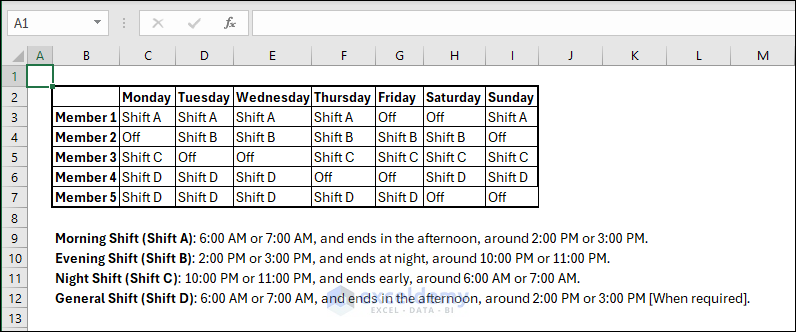
Hello SHIVAM
Thanks for your comment. To create a shift scheduler for a 5-member team with the specified shifts and off days, you can follow these steps:
Here is an example of how you could structure the scheduler:
Hopefully, the idea will help you; good luck.
Regards
Lutfor Rahman Shimanto
ExcelDemy
Hello CHARLIE
Thanks for your comment. The existing article’s date picker displays the date based on the date order of the Machine (Windows, Mac or Linux). However, you wanted to modify the VBA code to adjust the date format to match the desired month/day/year (American format) for both the calendar display and input into the cell. Thus, the idea will ensure consistency in date formats between the calendar view and the input into the cell.
To do so, you only need to modify the existing sub-procedure named Create_Calender by replacing it with the following.
Excel VBA Sub-procedure:
I hope you have found the idea helpful. Stay blessed.
Regards
Lutfor Rahman Shimanto
Excel & VBA Developer
ExcelDemy
Hello SHIQIANG
Thanks for sharing your problem. Typically, we are unable to perform such tasks in Excel. However, you can try using an Excel VBA Sub-procedure I have developed. It will display all the color indexes of the selected cells in the Immediate Window. The idea works perfectly if background is set manually or only one conditional formatting rule is applied in a cell. You can easily modify the formula for multiple conditional formatting rules based on your needs.
OUTPUT Overview:
Excel VBA Code:
Reach out again if you have any further queries. Hopefully, the idea will help you; good luck.
Regards
Lutfor Rahman Shimanto
Excel & VBA Developer
ExcelDemy
Hello NADHAY SARY
Thanks for visiting our blog and sharing your requirements. You wanted a Dynamic Leaderboard that updates automatically when the Average Sales will be changed.
OUTPUT Overview:
I am delighted to inform you that I have developed an Event Procedure and Sub-procedure using VBA to fulfil your goal.
Excel VBA Code:
Follow the steps: Right-click on the sheet name tab >> View Code >> Paste the given code in the sheet module >> Save >> Return to the sheet and make your desired changes.
Hopefully, the code will help you in reaching your goal.
Regards
Lutfor Rahman Shimanto
Excel & VBA Developer
ExcelDemy
Hello KARAN
Thanks for reaching out and posting such an interesting comment. Yes, you can manually specify holidays using the NETWORKDAYS.INTL function to customize which days are considered weekends and also lets you include specific holidays.
In your case, the first and second arguments in the formula are for the start and end dates; you can use 11 3rd arguments to consider only Sunday as the weekend. In the 4th argument, you insert the specified holiday.
I have developed a formula for January by focusing on your specified weekends and holidays.
Hopefully, the formula will help; good luck.
Regards
Lutfor Rahman Shimanto
ExcelDemy
Hello MATTEO
Thanks for visiting our blog and sharing your problem. Excel’s internal precision for numerical calculations can sometimes lead to unexpected results, especially when dealing with tiny or huge numbers.
To overcome your situation, you can combine the ROUND and CONVERT functions.
“mm” to “ft”:
“mm” to “in”:
Hopefully, the formula will help you overcome your situation; good luck.
Regards
Lutfor Rahman Shimanto
ExcelDemy
Hi ANDREW G,
Thank you very much for reading our articles.
You wanted to know a way to run the macro periodically without opening any file that will auto-refresh all the Excel files in a certain folder.
Here, I will discuss a way to fulfill your requirements. But to run a macro you need to open an Excel file and insert a macro in it. After that, the macro will refresh all your files in the mentioned folder. We will use the Task Scheduler feature of Windows to run the macro periodically.
Best Regards,
Alok Paul
Team ExcelDemy
Dear CARLOS,
Thank you for sharing your problem with us. To print 7 graphs as a single image:
Following the steps, we will get an image like the picture below.
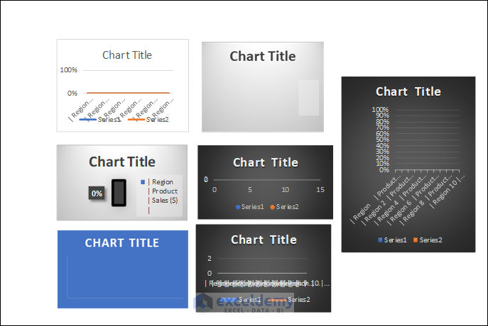
As a result, you will get all the graphs printed as a single image.
Regards
Wasim Akram
Team ExcelDemy
Hi Manisha
It is working fine for me and returning 10:16. Please give us more details about the formula and/or the dataset you are using.
Regards
Niloy
ExcelDemy
Hello,
Thank you for reaching out and sharing your experience. It seems like there might be an issue with the X-axis formatting.
To address the x-axis displaying as 1900, try the following steps:
Format X-Axis: After combining the scatter plots, right-click on the x-axis and select Format Axis. Check the settings to ensure the date format is correctly applied to your month values.
Date Formatting: Make sure that the Month values on the x-axis are recognized as dates. You may need to format the cells containing the monthly data as dates if they are not already.
Data Source: Double-check the data source for your scatter plot. Confirm that the Month values are correctly assigned to the x-axis.
X-Axis Labels: Ensure that the x-axis labels correspond to the Month values. Adjust the labels if necessary.
If you face the issues again, please provide more details about your data and the steps you followed, and I will do my best to help you.
Please let us know if your problem is solved or not.
Regards,
Bishawajit Chakraborty
ExcelDemy
Hi ED,
Thank you for your query. Unfortunately, directly importing your Yahoo Finance watchlist into Excel for stock details retrieval is not feasible due to technical limitations.
Reason:
Yahoo Finance watchlists are dynamic web pages primarily rendered by JavaScript, while Excel’s Data > From Web feature captures static HTML snapshots. This fundamental difference prevents Excel from capturing the interactive and user-specific nature of watchlists.
As an alternative solution, I recommend downloading the template from this link. Add your company names from the watchlist to this template. This template facilitates tracking and decision-making for your listed stocks within Excel.
We trust that this solution aligns with your interests and needs.
Best regards,
Ishrak Khan
ExcelDemy
Hi JAMES MARTIN,
Thank you for your positive feedback and for taking the time to recreate the example from the article. I’m glad you found the non-VBA REGEX example useful for your learning. I rechecked the process, and it worked fine for me. Did you recreate the example on our provided Excel file or try it on another workbook? For our provided workbook, if you want to recreate another named range, then you might need another name or a space, as you mentioned. However, it’s always helpful to receive feedback. If you have any further questions or suggestions, feel free to let us know. Your input is appreciated!
Regards
Rafiul Hasan
ExcelDemy
Hi DINESH,
Thanks for your comment. You can use the VBA code given below for the desired output.
I hope this user-defined function will solve your problem. Please let us know in the comment section if you have any other queries.
Regards
Maruf Hasan
ExcelDemy
Hi ISRAVEL,
To achieve this in Excel, you can use the COUNTIF function to count the occurrences of each number and then check which numbers occur more than twice. Here’s how you can set up your Excel sheet:
Assuming your numbers are in column A starting from A2, you can use the following formula in another cell to get the count of numbers that appear more than twice:
=COUNTIF(A:A, A2)Drag down this formula for each number in your list. This will give you the count of each number.
Then, you can use another column to check if the count is greater than 2:
=IF(B2>2, "More than two", "Not more than two")Drag this formula down for each number in your list.
This setup will give you a clear indication of which numbers occur more than twice in your list.
I hope this comment will help you get your required output. Please let us know in the comment section if you have any other queries.
Regards
Maruf Hasan
ExcelDemy
Hello OLIVER,
I hope you are doing well. Thank u for your query. Well, you can use the below formula to extract only the minimum value in the same cell.
=MIN(IFERROR(VALUE(MID($B$4:$B$8, FIND(":", $B$4:$B$8) + 1, LEN($B$4:$B$8))), ""))Note: Change the range (B4:B8) according to your dataset.
Hope this information will help you. Please let us know if there is any further query in the comment section.
Best Regards,
Afrina Nafisa
Exceldemy
Hi Kim, thanks for reaching out. Here’s a solution to your query to run the VBA code from the command prompt.
Here, I have used the VBA code shown in Method 4 of this article. The name of this macro is “Sheet3.SortPivotTableByValues” according to this article. Use it in your workbook and modify it according to your references.
Now, create a Notepad/Text document file and copy the following code in it. Change the file location and macro name if needed. Keep in mind that this macro was written in a sheet. So the sheet name should be added before the name of the Sub procedure.
Now, save the file as a .vbs extension file. In this case, I named it RunMacro.vbs.
After that, open the Command Prompt or cmd.exe. Press Windows + R buttons and type cmd in the Run dialog box and click OK.
The Command Prompt will appear. Copy and paste the following line and press Enter:
cd "C:\Users\DELL\Desktop”After that, copy and paste the following code in the next line and press Enter.
cscript RunMacro.vbs
Finally, your .xlsm file will open with the Pivot Table sorted. Hope this helps.
Regards
Meraz Al Nahian
ExcelDemy
Hi Chua!
It brings me great joy to know that you found our advice helpful. You are most welcome. As for troubleshooting your problem, it would be best if you could provide us with the Excel file. However, you could use the following steps to try to solve your problem on your own.
If your problem is not yet solved, please join our ExcelDemy Forum and post this problem with your Excel file attached to it.
Regards,
Nafis
ExcelDemy
Dear MARCOS,
Thank you for your query regarding the convertible bond pricing model presented in this article. Your query is valid, convertible bonds are bonds with the option to be converted into common stock. The conversion price refers to the price per share at which a convertible security (such as corporate bonds) can be converted into common stock.
The formula for conversion pricing is:
Conversion Price = Market Price of Convertible Bond / Conversion RatioTo find the conversion price, you need the “Conversion Ratio”, which is the number of shares that investors receive upon conversion. You can divide the Bond Value (C17) by the Conversion Ratio (C18) to find the Conversion Price (C19) as illustrated below.
I hope this clarification is helpful. If you have any further questions, please feel free to ask.
Kind Regards,
Sumaiya Mirza
ExcelDemy
Dear DORABABU
Thank you for your comment and your insightful observation. You are correct in pointing out that making prepayments towards the principal amount of a home loan can indeed result in a reduction in the total number of EMIs. This is an important consideration and can have a significant impact on the overall loan repayment timeline.
To incorporate this feature into the home loan EMI calculator, you can make the following adjustments to the existing formula:
Update Total Number of Months (N):
Instead of fixing the total number of months as G4×12, you can dynamically adjust it based on the prepayments made. You can introduce a new variable, say M, representing the total number of months after considering prepayments. The formula for M would be:
M=G4×12−Number of Prepayment MonthsModify the PMT Function for EMI Calculation:
Update the formula for EMI calculation (in cell C7) to reflect the adjusted total number of months (M):
=ABS(PMT(E4/12,M,F7))By making these changes, the calculator will dynamically adjust the total number of EMIs based on the prepayments made, providing you with a more accurate representation of the impact of principal payments on the loan tenure.
I hope this addresses your query. If you have any further questions or if there’s anything else you’d like to discuss, please feel free to ask.
Best Regards
Sumaiya Mirza
ExcelDemy
Dear Khristine,
Thank you for your comment. I have made some modifications to the code. Now, when you run it, a file picker dialog box will appear, allowing you to select a file. Once you’ve chosen the file, the Outlook app will open and a new email will be generated with the file attached. You can then manually send the email at your convenience. Here is the updated code:
I hope it will do the job for you.
Regards
Aniruddah Alam
ExcelDemy
Hello Miriam,
Thank you for sharing your problem with us. We are sorry you’re experiencing issues with the Excel VBA script for getting cell color.
Here are a few steps you can take to address the problem:
Please let us know if your problem is solved or not.
Regards,
Bishawajit Chakraborty
ExcelDemy
Hello ROSEMARIE OLIVERA,
Thanks for your response. Yes, you can apply the CELL function to the filtered table.
Regards
MD Naimul Hasan
Hello HANS ENGELS,
Thanks for your query. To extract data from the website to Excel automatically when the website requires login credentials, you must apply web scrapping techniques and automation tools.
First, you need to understand the web structure of that website and then use web scraping tools to get access to that website and extract data based on your needs.
Regards
MD Naimul Hasan
ExcelDemy
Hi Sandhya,
You can add 45 days with the invoice date and use it as a replacement for TODAY() in any of the formulas from above. Or, you can use a simple IF formula.
Here is an example, the invoice date is in cell C13. Use the formula:
=IF(C5>$C$13+45,"Overdue","Not Overdue")Make sure to use the correct reference style if you intend to drag the fill handle.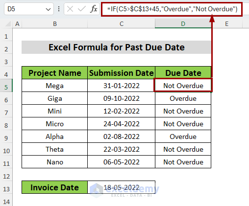
Regards
Abrar-ur-Rahman Niloy
ExcelDemy
Dear NORTH80,
Thank you very much for reading our articles.
You have mentioned that, when pulling historical dividend information you faced a problem. The problem is:
“Expression.Error: The column ‘Dividends’ of the table wasn’t found.
Details:
Dividends”
Here is the modified query code to solve the mentioned problem.
If you face further problems, please write in the comment box.
Best Regards,
Alok Paul
Team ExcelDemy
Hello VARUN
Thanks for reaching out and sharing your requirements. Your appreciation means a lot to us.
Yes, We can provide information on the Indian stock market with charts in dollars (INR) instead of dollars ($).
You can download this template below for your help. Additionally, I’m also writing down the steps so that you can modify it yourself.
Download Excel file: Track-Indian-Stock-Market.xlsx
Use these steps for indian stock market tracking:
Repeat the same process for other columns where necessary till J or Beta Column.
To update the format of Our Stock information section (Column K to P), follow these steps:
It will apply the same currency format to the applied range. Use the same process for Column O and P.
To update the format with Conditional formatting of Current Investment Column, copy the formatting of Changes (INR) column using Format Painter and paste it. It will automatically update both currency format and conditional formatting.
Note: The charts will update automatically.
Hope this helps you out.
Regards,
Ishrak Khan
ExcelDemy
Hi Zafar Iqbal,
In response to your request for some data entry work files, we have sent a PDF file for you to practice. Kindly check your email. You can also download the practice file provided with the article. Stay connected with ExcelDemy.
Regards
Rafiul Hasan
ExcelDemy
Hi Laurie!
It feels good to know that you found our content understandable. Judging from you query, I think you want a continuing compound interest formula where the loan doesn’t have a specific term/year.
The term continuous compound interest is used to emphasize the continuous compounding of interest, as opposed to discrete compounding periods. Here, the compounding frequency becomes infinite, resulting in a continuous growth formula. Let us look at the formula below:
A=P0ert
Where,
For example, if you invest $1,000 at an annual interest rate of 5% continuously compounded for 2 years, the future value can be calculated using the continuous compounding formula.
Regards,
Nafis
ExcelDemy
Hello LAKSHMI,
I hope you are doing well. Thank you for your query. You can combine sheets row-wise using the VBA code provided in the first method of this article. (Merge Data Sets from Multiple Sheets into One Sheet with VBA Row-wise). Once you go through this method of merging data sets, you will know where to change the code as the details are written in the “Note”.
Best Regards,
Afrina Nafisa
Exceldemy
Hello Lea, thanks for reaching out. Here’s a solution for your query.
Procedure:
Regards
Meraz Al Nahian
ExcelDemy
Hello ODMA
Thanks for reaching out and sharing your queries. The previous question by ABIGAYLE PAULSON was to automate the idea that the filtering algorithm will be applied if the drop-down list in Sheet8 is changed. After analyzing your requirements, I understand that you do not want to use the filter algorithm if the drop-down is empty.
I have developed an Excel VBA Worksheet_Change Event that will fulfil your goal. All you need is to paste the following code in the sheet module of Sheet8 (the sheet that contains the drop-down).
Excel VBA Event Procedure:
OUTPUT Overview:
Hopefully, the event procedure will help; good luck.
Regards
Lutfor Rahman Shimanto
Excel & VBA Developer
ExcelDemy
Hello POOJA
Thanks for reaching out and sharing your requirements with such clarity. The problem you want a solution for can quickly be developed using several Excel VBA Sub-procedures, Event Procedures, and a UserForm.
Here is an algorithm you can follow:
OUTPUT Overview:
Regards
Lutfor Rahman Shimanto
Excel & VBA Developer
ExcelDemy
Hello ANDREW
Yes, that’s correct. In both methods described in the article, you would need to open the file containing the macro to auto-refresh the target Excel files. However, once the macro is executed, it will open and refresh the specified Excel files without manually opening them individually.
Regards
Lutfor Rahman Shimanto
ExcelDemy
Hello GRAHAM
Thanks for reading our blogs and sharing your requirements. You wanted to display the range-converted images horizontally in the email body. This can be achieved by slightly modifying the article’s Excel VBA code.
OUTPUT OVERVIEW:
Excel VBA Code:
I have another present for you. If you ever want to attach the images generated from the selected ranges, you can use the following code:
Hopefully, the codes will help in various situations. I have also attached the solution workbook; good luck.
DOWNLOAD SOLUTION WORKBOOK
Regards
Lutfor Rahman Shimanto
Excel & VBA Developer
ExcelDemy
Hello RAMI
Thanks for visiting our blog and sharing your queries. You want to create multiple stopwatches in a sheet. Of course, the requirement is very much achievable.
I have displayed four stopwatches in the B4, F4, B15, and F15 cells.
OUTPUT OVERVIEW:
Follow these steps:
I hope you have learned how to create multiple stopwatches in a sheet. I am also attaching the solution workbook for better understanding; good luck.
DOWNLOAD SOLUTION WORKBOOK
Regards
Lutfor Rahman Shimanto
Excel & VBA Developer
ExcelDemy
Hello SINTA R
Thanks for reaching out and sharing your queries. The formula you have mentioned is almost correct. However, you miss to insert the <> sign somehow in your formula.
You can apply the following formulas:
For Important & Urgent:
=IFERROR(INDEX($C$4:$C$30,SMALL(IF((LEN($C$4:$C$30)<>0)*($D$4:$D$30="Yes")*($E$4:$E$30="Yes"),ROW($C$4:$C$30)-ROW($C$3),""),ROW(C4)-ROW($C$3))),"")For Important & Not Urgent:
=IFERROR(INDEX($C$4:$C$30,SMALL(IF((LEN($C$4:$C$30)<>0)*($D$4:$D$30="Yes")*($E$4:$E$30="No"),ROW($C$4:$C$30)-ROW($C$3),""),ROW(C4)-ROW($C$3))),"")For Not Important & Urgent:
=IFERROR(INDEX($C$4:$C$30,SMALL(IF((LEN($C$4:$C$30)<>0)*($D$4:$D$30="No")*($E$4:$E$30="Yes"),ROW($C$4:$C$30)-ROW($C$3),""),ROW(C4)-ROW($C$3))),"")For Not Important & Not Urgent:
=IFERROR(INDEX($C$4:$C$30,SMALL(IF((LEN($C$4:$C$30)<>0)*($D$4:$D$30="No")*($E$4:$E$30="No"),ROW($C$4:$C$30)-ROW($C$3),""),ROW(C4)-ROW($C$3))),"")OUTPUT OVERVIEW:
Hopefully, you have found your solution. I have also attached the solution workbook for better understanding; good luck.
DOWNLOAD SOLUTION WORKBOOK
Regards
Lutfor Rahman Shimanto
ExcelDemy
Hello DORY
Thanks a Ton! for your nice words. Your appreciation means a lot to us.
You would like to copy only a specific range from the source workbook. I am presenting an Excel VBA Sub-procedure that will fulfil your requirements.
OUTPUT OVERVIEW:
Excel VBA Sub-procedure:
Hopefully, you will like the example and the sub-procedure. Good luck.
Regards
Lutfor Rahman Shimanto
Excel & VBA Developer
ExcelDemy
Hello JAMES
Thanks for reaching out and sharing your queries. To return the text value of two cells in different columns if they match, you can combine the EXACT, IF and ISTEXT functions.
Excel Formula:
=IF(AND(ISTEXT(A2), ISTEXT(B2), EXACT(A2, B2)), A2:B2, "No Match")So, in simpler terms, the formula checks if both cells A2 and B2 contain text and if the text in both cells is the same. If they are, it returns the values from cells A2 and B2 together. If not, it returns “No Match”.
OUTPUT:
Hopefully, the idea will help you; good luck.
Regards
Lutfor Rahman Shimanto
ExcelDemy
Hello BRYAN
Thanks for visiting our blog. All the methods described in the article are working perfectly on our end. It is important to remember the intended effect you want to see when you have printed the sheet.
OUTPUT OVERVIEW:
So, I recommend you reread the article; good luck.
Regards
Lutfor Rahman Shimanto
ExcelDemy
Hello GARY SHERMAN
Thanks for reaching out and sharing your problem. You want to find the total number of sheets for each material type. To do so, you can use the SUMIF function to reach your goal.
Follow these steps:
As a result, you will see an output like the following image.
Hopefully, the idea will help; Good luck.
Regards
Lutfor Rahman Shimanto
ExcelDemy
Dear Kelly
Thank you so much for your kind words! It’s fantastic to hear that our tutorial has been helpful to you. You’ve already made quite an impact in your new role, becoming the Excel expert in your office – that’s quite an accomplishment!
Let us know if you ever need more help with Excel or anything else. We’re here for you. Best wishes for your continued success at the mom & pop shop!
Best Regards
Lutfor Rahman Shimanto
ExcelDemy Team
Hello CHRISTOF
Thanks for sharing your queries. Depending on your OS Version, the User-defined functions may give this type of error. Ensure you run a 64-bit Windows, and let us know if you still face the error.
Regards
Lutfor Rahman Shimanto
ExcelDemy
Hi Karthick
Thank you for reaching out with your inquiry! Designing a shift schedule for a 4-member team roster with diverse shift patterns can be challenging.
Each shift, A, B, C, and D, has a schedule for weekdays, weekends, and special arrangements on Wednesdays. Setting these parameters upfront allows you to assign team members to their shifts more efficiently.
On Wednesdays, all four members are active but in different roles. It would be best if you had a flexible framework to handle this. One idea is to create a dynamic formula that adjusts shift assignments based on the day of the week and specific requirements. This might involve using conditional logic to distribute team members across day and night shifts, ensuring we have enough coverage while using resources effectively.
Don’t forget to explore the resources in the article, including the practice workbook, to gain hands-on experience with building and refining your shift scheduler. Good luck.
Regards
Lutfor Rahman Shimanto
ExcelDemy
Hello ERAL
Good to see you again. You wanted shifts like, Instead of using D1, D2, D3, D4, OFF, A1, A2, A3, OFF, is it possible to use just like this only D, D, D, D, OFF, A, A, A, OFF. Technically, it is impossible without VBA, but I have found a trick to reach your goal. I have used extra spaces in the Settings_Shift_Legend to make the shifts unique.
OUTPUT OVERVIEW
Hopefully, I will like the idea. I have attached the solution workbook to help you understand better; good luck.
Download Solution Workbook
Regards
Lutfor Rahman Shimanto
ExcelDemy
Hello FRED FUTCH
Thanks for sharing your problem. You might be experiencing some formatting issues in Excel when inputting numbers.
Ensure that the cells where you are typing numbers are formatted as General or Number. Sometimes, Excel may automatically apply a different format if it detects a specific pattern in the data.
Sometimes, Excel’s behaviour can be influenced by the regional settings on your computer. Make sure that your computer’s regional settings are configured correctly.
Hopefully, the idea will help in your situation; good luck.
Regards
Lutfor Rahman Shimanto
ExcelDemy
Hello FRANKY LAM
Thanks for visiting our blog and sharing your problem. Based on your problem, it seems the VBA User-defined function named Code128 is not recalculating on your system.
So, you can try forced fully recalculating using the CalculateFull property of the Excel Application.
Follow these steps: Right-click on the sheet name tab >> Click on View Code >> Paste the following code in the sheet module and Save:
Hopefully, the idea will help you good luck.
Regards
Lutfor Rahman Shimanto
Excel & VBA Developer
ExcelDemy
Hello Samir
Thanks for visiting our blog and posting an interesting comment. You want to convert a number (e.g., 10245) into a string where each digit of the number is represented by its word form (e.g., “One Zero Two Four Five”).
I am delighted to inform you that I have developed an Excel VBA User-defined function named NumberToString to fulfil your goal. I am using the function in a Sub-procedure. However, you can also use it in Excel cells like other worksheet functions.
OUTPUT OVERVIEW:
Excel VBA Code:
Hopefully, the user-defined function will help you reach your goal; good luck.
Regards
Lutfor Rahman Shimanto
Excel & VBA Developer
ExcelDemy
Hello ASNATH
Thanks for reaching out and posting your comment. You want to know how to use the COUNT, IF and AVERAGE functions in a formula. I am presenting an example where I will form a formula using these functions.
OUTPUT OVERVIEW:
Suppose your dataset has Employee ID, Name, Department, Age, and Salary columns. You want to find out the average salary based on department. You can get the result using only the AVERAGEIF function, but if the department does not exist, it will provide a #DIV/0! Error. So, to handle this type of situation, you can combine COUNT, IF, SUM and AVERAGE functions:
Hopefully, the idea will help you. Good luck.
Regards
Lutfor Rahman Shimanto
ExcelDemy
Hello JAN ZÁKOSTELSKÝ
Thanks for reaching out and sharing your problem. You want to compare two Excel rows: one that remains constant and another that changes. You need to receive an email whenever a number in any cell of the changing row becomes lower than the value in the corresponding cell of the constant row.
I am delighted to inform you that I have developed an Excel VBA Sub-procedure and an Event Procedure. These will fulfil your requirements.
Follow these steps:
Hopefully, the idea will help you; good luck.
Regards
Lutfor Rahman Shimanto
Excel & VBA Developer
ExcelDemy
Hello VICTORIA SHARP
Thank you for reaching out and sharing your requirements. Based on your comment, it seems like you’re looking for a dynamic link between your Excel sheet and Word document to ensure that any updates in the Excel sheet reflect immediately in the Word document.
The solution provided in the article serves this purpose quite effectively. Using the Mail Merge feature in Word, you can connect your Excel sheet (containing the Conflict of Interest Register data) and your Word document.
So, do not hesitate to follow the steps outlined in the article to establish the connection between the two. Once set up, any changes you make to the Excel sheet will automatically propagate to the Word document when you update the merge fields. This way, you can maintain an accurate and current Conflict of Interest Register without manual effort. Good luck.
Regards
Lutfor Rahman Shimanto
ExcelDemy
Hello ANUPAM
Thanks for reaching out and sharing your queries. You not only want to count total links but also to display cells containing links.
I am delighted to inform you that I have an Excel VBA sub-procedure that will fulfil your goal. The code will display the total links in a MsgBox and show all the cells containing links in the Immediate window.
OUTPUT OVERVIEW:
Excel VBA Sub-procedure:
Hopefully, the code will help you; good luck.
Regards
Lutfor Rahman Shimanto
Excel & VBA Developer
ExcelDemy
Hello VIKAS
Thanks for reaching out and sharing your queries. You wanted to count the total number of named ranges in a workbook.
I am delighted to inform you that I have developed an Excel VBA sub-procedure to display the total number of named ranges in an Excel MsgBox.
OUTPUT OVERVIEW:
Excel VBA Sub-procedure:
Hopefully, the code will help you. Good luck.
Regards
Lutfor Rahman Shimanto
Excel & VBA Developer
ExcelDemy
Hello EXCELFLASH
Thanks a ton for taking the time to dive into our article and sharing your thoughts! We’re thrilled to hear that you found it excellent overall – that means a lot to us.
We’re sorry you encountered an issue with the formula from method 1. After investigating, we discovered that you are correct about the line spacing and quotation marks issues in that formula when copying.
We’ve updated the article, so feel free to retry it. Hopefully, this time around, you won’t encounter the same hassle with the formula. Let us know if you have any further questions or suggestions.
Regards
Lutfor Rahman Shimanto
ExcelDemy
Hello BHARATH L
Thanks for your nice words. Your appreciation means a lot to us. You wanted to mention a series of numbers for every copied row. In your words, if you have copied 50 columns using the code, you need to mention 1 to 50 numbers in each row.
I am delighted to inform you that I have developed an Excel VBA sub-procedure to fulfil your requirements. I have modified the existing article code and made it an advanced version.
OUTPUT OVERVIEW:
Advanced Excel VBA Code:
Hopefully, the code will fulfil your goal. Good luck.
Regards
Lutfor Rahman Shimanto
Excel & VBA Developer
ExcelDemy
Hello TIM
Thanks for reaching out and sharing your query. You want an Excel VBA code that works perfectly for multiple columns and rows of checkboxes. I am presenting an enhanced VBA sub-procedure that may help you.
OUTPUT OVERVIEW:
Enhanced Excel VBA Code:
Hopefully, the sub-procedure will reduce your hassle. Good luck.
Regards
Lutfor Rahman Shimanto
Excel & VBA Developer
ExcelDemy
Hello KHALED
Thanks for your nice words. Your appreciation means a lot to us. You only want to get the city name from lat and long values.
I am delighted to inform you that I have developed another VBA User-defined function named ExtractCityNames that will extract the city names by taking input from the User-defined function mentioned in this article.
Follow these steps:
Things to Remember: The return time can be longer than usual as we use complex Excel VBA User-defined functions.
I am attaching the solution workbook for better understanding. Hopefully, the idea will fulfil your goal. Stay Blessed.
DOWNLOAD SOLUTION WORKBOOK
Regards
Lutfor Rahman Shimanto
Excel & VBA Developer
ExcelDemy
Hello Abdul
Thanks for reaching out and posting your comment. You want to highlight the scenario where a student, Raju, fails in one subject out of five but still manages to achieve a high percentage overall due to scoring well in the remaining subjects.
Basically, you want to ensure that Raju isn’t labelled a failure just because he fails one subject. In your view, Raju’s overall performance across all subjects should involve when determining his pass/fail status, not just the grade in one subject.
Hopefully, you have found the idea helpful. Good luck.
Regards
Lutfor Rahman Shimanto
ExcelDemy
Hello NIKKI
Thanks for reaching out and sharing your queries. You want to automatically fill a cell background to yellow anytime a change is made to the data inside the cell.
I am delighted to inform you that I have developed an Excel VBA change event that will fulfil your goal. To demonstrate, assume you want to auto-fill a cell in column A to yellow.
To do so, open the sheet module => Insert the following code and Save.
Now, return to the sheet and change some cell values in column A to get an output like the following GIF.
Hopefully, the idea will help you. Good luck.
Regards
Lutfor Rahman Shimanto
Excel & VBA Developer
ExcelDemy
Hello SCOTT
Thanks a lot for your kind words. You want to specify a particular column from a table in Excel VBA ComboBox’s RowSource property.
Output Overview:
Let’s assume you have a table named Data in the sheet Database with several columns, and you want to populate your ComboBox with the values from a specific column, let’s say the Project column.
You can use the following format for the RowSource property: =Database!Data[Project]
Hopefully, the idea will help. I have also attached the solution workbook for better understanding. Good luck.
DOWNLOAD SOLUTION WORKBOOK
Regards
Lutfor Rahman Shimanto
Excel & VBA Developer
ExcelDemy
Hello ARONN
Thanks for reaching out and sharing your requirements. You want to link a checkbox directly to another one with no cell reference.
I am delighted to inform you that I have developed an Excel Event Procedure that will fulfil your goal.
Output Overview:
If you check the first box, a linked check box (second check box) will also be checked or vice versa.
Follow these steps:
Hopefully, the idea will help you. I have attached the solution workbook for better understanding. Good luck.
SOLUTOIN WORKBOOK
Regards
Lutfor Rahman Shimanto
Excel & VBA Developer
ExcelDemy
Hello RENE
Thanks for reaching out and sharing your problem. You have observed that the formula works for the first eight rows. When you expand to include cells B5:B144 and C5:C144, it returns #N/A. However, our machine works perfectly fine, even though we work with an extensive range. The FILTER function is only available in Excel for Microsoft 365 and Excel 2021. Assuming you are using one of these versions.
To resolve your problem, double-check the references in the formula to ensure they correspond to the correct columns and cells. Confirm that the formula is entered correctly without any typos or syntax errors. Good luck.
Regards
Lutfor Rahman Shimanto
ExcelDemy
Hello JITHU
Thanks for reaching out. You are right about the file not allowing the opening of macros. The password is recovered using the Zip Tool, which will not let you open macros. In the article, the writer has demonstrated the file as a macro-free file when using the Zip tool. That’s why when changing back to the file type Zip to Excel, the .xlsx is used.
If you are working on a macro-enabled file when recovering a password using Zip Tool, change the file’s extension (when changing the file type Zip to Excel) to .xlsm instead of .xlsx.
Regards
Lutfor Rahman Shimanto
ExcelDemy
Hello DENNIS IVAN FORD
For the Time_Box to work properly, paste the following code in the UserForm.
Through this code, the UserForm will be able to add time with a date when the Add Time check box is ticked.
Download the practice workbook provided in the article for better understanding. Good luck.
Regards
Lutfor Rahman Shimanto
ExcelDemy
Hello DENNIS IVAN FORD
Thanks for your comment. For the Month_Box to work properly, paste the following code in the UserForm.
Additionally, you can remove the Option Explicit statement at the beginning when declaring initial variables.
The article has been updated. So, I recommend you to go to the article again. Good luck.
Regards
Lutfor Rahman Shimanto
ExcelDemy
Hello SHASHA
Thanks for reaching out and posting your question. I would say yes, you have found the solution to your problem. You can fix this problem by changing the date format in your computer’s date and time settings. Change the date format to your desired one.
However, I am delighted that I have an ultimate solution. I am presenting an Excel VBA sub-procedure that will display the date format based on the PC date & time setting.
OUTPUT Overview:
All you need to do is replace the existing Create_Calender sub-procedure with the following enhanced sub-procedure.
Hopefully, the idea will help you good luck.
Regards
Lutfor Rahman Shimanto
Excel & VBA Developer
ExcelDemy
Hello Karan
Thanks for sharing your problem. The practice workbook attached to the article should be usable in Windows 11 OS.
As the Excel file is macro-enabled, check your Excel security settings: Go to Excel Options > Trust Center > Trust Center Settings > Macro Settings, and enable macros if they are disabled.
Besides, ensure that the Code 128 font is correctly installed on your system.
Hopefully, these actions will resolve your issue. Good luck.
Regards
Lutfor Rahman Shimanto
Excel & VBA Developer
ExcelDemy
Hello Jon Jacobson
Thanks for your nice words. The code and font work perfectly fine in our machine for numbers greater than 999. See the following Image,
You can test the barcodes shown in the image using your barcode gun. On our end, we have found the original text accurately.
It is impossible to thoroughly observe your problem remotely and not glance at your machine. Make sure you have installed the Code 128 barcode font properly. You can check the scanner manual for specific settings related to Code 128 barcodes.
If you still face this type of problem, you can share the issue within the ExcelDemy Forum with details of your machine. Stay blessed.
Regards
Lutfor Rahman Shimanto
Excel & VBA Developer
ExcelDemy
Hello TH
Thanks for reaching out and sharing your requirements. You wanted a roaster including D1, D2, DN, N1, N2, and O to rotate full month and continue next month.
I am delighted to inform you that I have created a roaster to fulfil your goal. So, follow these:
Return to the sheet, and use the file like the following GIF.
Hopefully, the idea will work for you. I am attaching the solution workbook for better understanding. Good luck.
DOWNLOAD SOLUTION WORKBOOK
Regards
Lutfor Rahman Shimanto
ExcelDemy
Hello KIMHONG
Thanks for sharing your query. In your case, an employee works 11 hours and starts working at 5:30 AM. If the overtime is between 0 and 15 minutes, you wanted a formula that returns 0 minutes. If it’s 15 minutes or more, it’s considered as 30 minutes.
You can achieve the goal by developing a formula using the IF and TIME functions. Follow these steps:
Hopefully, the idea will help. Good luck.
Regards
Lutfor Rahman Shimanto
ExcelDemy
Hello NC
Thanks for sharing your requirements. You wanted a setup not to overwrite the existing entry but to create a new entry timestamp when an item is checked in or out more than once.
I am delighted to inform you that I have developed an Excel VBA Sub-procedure to fulfil your requirements. So, follow these steps:
After inserting the bar code and running the sub-procedure, you will see an output like the following GIF.
Hopefully, the idea will help you to reach your goal. I have attached the solution workbook. Good luck.
DOWNLOAD SOLUTION WORKBOOK
Regards
Lutfor Rahman Shimanto
Excel & VBA Developer
ExcelDemy
Hello KAJA POHAR
Thanks for your compliments. Your appreciation means a lot to us. You wanted to work with a read-only Excel file; however, you had issues with the existing VBA code.
I am delighted to inform you that I have developed an Excel VBA Sub-procedure by modifying the existing VBA code. The main idea behind the sub-procedure is it changes the File Access property to xlReadWrite, and before closing, it changes the File Access back to xlReadOnly.
Follow these steps:
As a result, you will see an output like the following GIF.
Hopefully, the idea will help you to reach your goal. Good luck!
Regards
Lutfor Rahman Shimanto
Excel & VBA Developer
ExcelDemy
Hello L. O.
Thanks for reaching out and sharing your problem. You are facing difficulties with including a heading in a chart, and those headings affect the graph’s appearance.
As the headings are treated as zeros, you can exclude them from the data by combining the IF, ISNUMBER and NA functions. The formula structure can be like the following:
This formula checks if the value in cell A2 is a number. If it is, it includes the value. Otherwise, it returns #N/A. The #N/A values will be ignored in the chart, and the line won’t connect to them.
Instead of a scatter plot, you might consider using a line chart or other chart types that suit your needs better. Line charts, for example, automatically ignore #N/A values and don’t connect them.
Hopefully, the ideas will help you to overcome your situation. Good luck!
Regards
Lutfor Rahman Shimanto
ExcelDemy
Hello NUNOF
Thanks for your beautiful words. Your appreciation means a lot to us. We are delighted to know you have learned a lot from our blog.
The issue you describe hampers performance for sure in such scenarios. I have gone through the article and also investigated your problem. What I have found: Perhaps you are calling your desired macro within another worksheet event like Worksheet_Calculate instead of the Worksheet_Change event of cell $K$10, which results in calling the macro unintentionally.
When the cell values change by formulas, the Worksheet_Change event will not trigger. So, call your macro or sub-procedure within a change event. In your case, the code within the sheet module can be like the following:
Hopefully, you have found the idea to overcome your situation. Good luck!
Regards
Lutfor Rahman Shimanto
Excel & VBA Developer
ExcelDemy
Hello RAY
Thanks for reaching out and sharing your query.
Unfortunately, the Paste Special feature is unavailable in Excel Online compared to the desktop version.
There is a list of missing features that you will also not find in Excel Web:
Hopefully, the answer and list will help you regarding your queries. Good luck!
Regards
Lutfor Rahman Shimanto
ExcelDemy
Hello RAMNATH TAKIAR
Thanks a Ton! for your nice words. Your appreciation means a lot to us. Thank you once again for sharing your expertise with our ExcelDemy blog!
The extra values you have added prove effective. We appreciate you sharing your program with us, and we believe it will be valuable to others who visit our blog.
To generate even 500 random samples from the selected population of 200:
OUTPUT OVERVIEW:
Excel VBA Sub-procedure (Contributed by RAMNATH TAKIAR):
Regards
Lutfor Rahman Shimanto
Excel & VBA Developer
ExcelDemy
Hello ALEX
Thanks for your nice words. Your appreciation means a lot to us.
You are facing a difficulty like when you press the enter button on cell D5 with the formula, the barcode changes. It’s different from the original one and can’t be scanned. Providing the ultimate solution without properly glancing at your problem is very hard. However, I am giving you some ideas that might be helpful.
Suggestions: Your issue concerns the font encoding or handling of the Code 128 font in Excel. Make sure that the Code 128 font is installed correctly on your system. Check the scanner manual for any specific settings related to Code 128 barcodes. Format the cell as Text when using the Code 128 barcode font with a custom VBA function to ensure accurate content and avoid unintended changes by Excel formatting rules.
You can also share your problem with more details in the ExcelDemy Forum. Good luck.
Regards
Lutfor Rahman Shimanto
ExcelDemy
Hello GSFRAGARO
Thanks for sharing your problem. You have encountered an issue like you have a string with two consecutive zeros, but the code generates an empty character. In Our machine, the code and font work perfectly fine if we have a string with two consecutive zeros. See the following Image,
The possible reason for the issue you encountered could be not using the Code 128 font. Maybe you are using some other barcode font. So, please ensure you are using the intended font. Good luck.
Regards
Lutfor Rahman Shimanto
ExcelDemy
Hello NURIT
Thanks for sharing another exciting problem. The issue is raised because the UDF (User Defined Function) is not re-calculating.
I am excited to let you know that I have resolved the issue by developing an Excel VBA Sub-procedure named ForcedReCalculation (responsible for application re-calculation).
OUTPUT OVERVIEW:
Follow these steps: Open the VBA Editor window => Right-click on the sheet module => Click on View Code => Replace the previous code with the following code => Save.
Hopefully, you have found your solution. I look forward to seeing you at the ExcelDemy Forum with another exciting problem. Stay blessed.
Regards
Lutfor Rahman Shimanto
Excel & VBA Developer
ExcelDemy
Hello JOHN
Thanks for sharing your query. You wanted to split strings within Excel cells that do not always have 3 words separated by commas. In contrast, there can be a string like one or at most three words like the following image. Besides, we must keep the cell empty if more than 3 words mean more than 2 commas exist.
I am delighted to inform you that I have developed two formulas. The first formula consists of the IF, LEN, SUBSTITUTE, TRIM, and MID functions. The other formula consists of the IF, LEN, SUBSTITUTE, TRANSPOSE, and FILTERXML functions.
OUTPUT OVERVIEW:
1. Using IF, LEN, SUBSTITUTE, TRIM, and MID functions
Follow these steps:
Step 1: Select cell C5, insert the given formula and drag the Fill Handle icon to E5.
Step 2: Select range C5:E5 and drag the Fill Handle icon to cell E10.
2. Using FILTERXML, TRANSPOSE, IF, LEN, and SUBSTITUTE functions
I am attaching the solution workbook for better understanding. I hope these ideas will help you to reach your goal. Good luck.
DOWNLOAD WORKBOOK
Regards
Lutfor Rahman Shimanto
ExcelDemy
Dear NURIT
It is good to see you again. Thanks for thanking me. Your appreciation means a lot to us.
You are right. When a cell background color is changed by conditional formatting, the cell color index remains xlColorIndexNone. When using conditional formatting to change the cell background based on a condition, it fetches the intended color, but the cell background is not changed ultimately.
SOLUTION to the Mentioned Problem: Remove the conditional formatting from the S8:AO43 range. Use an Excel VBA Event procedure that I developed to solve your problem. This event will ultimately change the background color based on the condition.
Follow these steps: Right-click on the sheet name tab => Click on View Code => Paste the code below in the sheet module, and Save => Return to the sheet and make changes to see the output like the following GIF.
Enhanced User-defined Function: I am delighted to share an Enhanced version of the previous sub-procedure.
Follow these: Hover over Insert => Click on Module => Paste the following code in the module => Save.
Finally, to calculate the sum, Select cell Q8 => Insert the following formula => Drag the Fill Handle icon to cell Q14.
Besides, I am presenting an sub-procedure that will display the color index of a selected cell.
A Friendly Suggestion: Dear Nurit, we are discussing a topic different from the article. So, another visitor may get confused. It would be great if you shared your problem through the ExcelDemy Forum.
I am also attaching the solution workbook for better understanding. Hopefully, this idea will help you reach your goal. Good luck.
DOWNLOAD WORKBOOK
Regards
Lutfor Rahman Shimanto
ExcelDemy
Hello ZAPPER
Thanks for reading ExcelDemy Blogs. You wanted a button to click and copy some sheets in a folder.
I am delighted to inform you that I have enhanced the sub-procedure so you will like it. The sub-procedure will create a folder dynamically, and the path will be the workbook path. Besides, it will handle errors as well. I have inserted a print icon and assigned the sub-procedure as follows.
OUTPUT OVERVIEW:
Enhanced Excel VBA Sub-procedure:
I am attaching the solution workbook for better understanding. Good luck.
DOWNLOAD WORKBOOK
Regards
Lutfor Rahman Shimanto
ExcelDemy
Hello MR MARTYN WILLIETS
Thanks for reaching out and sharing your requirements. You wanted to create a personal payment tracker sheet. To create such a sheet, we can work with fields like Date, Start Time, End Time, Total Paid Hours, Overtime Hours, Overtime Pay, Normal Hours Pay, and Total Pay. Assuming you get $76.5 for overtime hours and $51 for regular hours. I am delighted to share how you can create a sheet to fulfil your goal.
Overview of Personal Payment Tracker Sheet:
Follow these steps:
Step 1: Total Paid Hours
Select cell E3 => Insert the following formula => Drag the Fill Handle icon to cell E10.
Step 2: Overtime Hours
Select cell F3 => Insert the formula below => Drag the Fill Handle icon to cell F10.
Step 3: Overtime Pay
Choose cell G3 => Insert the formula below => Drag the Fill Handle icon to cell G10.
Step 4: Normal Hours Pay
Choose cell H3 => Insert the formula below => Drag the Fill Handle icon to cell H10.
Step 5: Total Pay
Choose cell I3 => Insert the formula below => Drag the Fill Handle icon to cell I10.
I am also attaching the solution workbook for better understanding. Hopefully, the idea will help you to reach your goal. Good luck.
DOWNLOAD WORKBOOK
Regards
Lutfor Rahman Shimanto
ExcelDemy
Hello ASIF MAHMOOD
Thanks for reaching out and sharing your requirements with such clarity. You wanted to know how to convert a string like 159.3 B into a regular unit format (for example, 159300000000.00).
I am delighted to inform you that I have developed an Excel VBA Event Procedure that will trigger when a value is inserted in a format like 13 B in column B and convert the values into a regular unit. Besides, I have developed an Excel formula to fulfil your goal using the TEXT and SUBSTITUTE functions.
OUTPUT OVERVIEW (Excel VBA Event Procedure):
Follow these steps:
Step 1: Right-click on the sheet name tab => Click on View Code.
Step 2: Hover over Insert => Click on Module => Paste the following code in the module => Save.
OUTPUT OVERVIEW (Using Excel TEXT and SUBSTITUTE Functions):
Follow these steps:
Step 1: Select cell C5 => Insert the following formula => Hit Enter.
Step 2: Drag the Fill Handle icon to cell C14 to copy the formula down.
I am also attaching the solution workbook for better understanding. Good luck.
DOWNLOAD WORKBOOK
Regards
Lutfor Rahman Shimanto
ExcelDemy
Hello GARY PHILLIPS
Thanks for reaching out and sharing your queries. You want to know how to use the Monthly Log presented in the article. Copy the drop-down of symbols and paste it in all the day cells. Choose the intended symbols using drop-down for all the day sections of the month. If a task is complete, mark it as Complete in the left section above the calendar.
You can easily use the Monthly Log like the following GIF.
Hopefully, the idea will help you. Good luck!
Regards
Lutfor Rahman Shimanto
Hello DAN H
Thanks for your nice words. Your appreciation means a lot to us. Thanks once again for sharing your requirements with such clarity.
You wanted to get an Excel VBA Sub-procedures or Excel VBA User-defined functions to calculate the distance between two addresses using Address String (for example, New York, Alaska) instead of Latitudes and Longitudes values.
I am delighted that I developed some Excel VBA User-defined functions to fulfil your requirements.
OUTPUT OVERVIEW:
Follow these steps:
Step 1: Hover over Insert => Click on Module => paste the following code in the module.
Step 2: Select cell C9 => Insert the following formula.
Step 3: Hit Enter to see the result in cell C9.
Step 4: Select cell C10 => Insert the following formula.
Step 5: Hit Enter to see the result in cell C10.
Things to Keep in Mind: Ensure to check Microsoft XML, v3.0 from the References – VBAProject window.
I am attaching the solution workbook. Hopefully, these user-defined functions will help you reach your goal. Good luck.
DOWNLOAD WORKBOOK
Regards
Lutfor Rahman Shimanto
Excel & VBA Developer
ExcelDemy
Hello BRIAN
Your appreciation means a lot us. Thanks for reaching out and posting a well-layout question. You encounter an issue with hidden columns and buttons that toggle between different sheet views. And you want to delete these buttons and the hidden column features. It isn’t easy to give an exact solution without the exact details of the worksheet views. However, I have some general ideas to help you with your problem.
First, identify the toggle buttons and go to sheet views, followed by view options. Later, delete that sheet view. Additionally, you remove the applied filters and groupings. Select the columns surrounding the hidden ones, right-click, and choose Unhide to ensure all columns are visible.
If you still have difficulties, you can share your problem in the ExcelDemy Forum with more detailed information. Good luck!
Regards
Lutfor Rahman Shimanto
ExcelDemy
Hello NURIT
Thanks for your nice words. Your appreciation means a lot to us. You wanted a VBA code that will ignore the text within a cell and sum only the number portion on that cell of the S8:AO43 range based on specific conditionally formatted colors.
I am delighted to inform you that I have developed an Excel VBA User-defined function to fulfil your goal.
OUTPUT OVERVIEW:
Excel VBA User-defined Function:
Follow these steps:
Step 1: Open the VBA Editor window => Hover over Insert and click on Module => Insert the code above in the module and Save.
Step 2: Select cell P20 => Insert the following formula => Hit Enter.
Hopefully, the idea will help you. Good luck.
Regards
Lutfor Rahman Shimanto
ExcelDemy
Hello BERNARD
Thanks for reaching out and posting your observation. The ZIP Tool method mentioned in the article can be applicable If you have a protected sheet within a workbook.
I have experienced the same error when the workbook is encrypted with a Password. But, if only a sheet is protected, the ZIP Tool works perfectly. When you preserve your workbook with an Encrypted Password, the ZIP Tool method will not work. So, use the VBA code to remove the password from the encrypted workbook. Good luck.
Regards
Lutfor Rahman Shimanto
ExcelDemy
Dear AVA
Your appreciation means a lot to us. Thanks for describing your problem with such clarity. You want a column of comments and a column of texts in which a comment was made (e.g. Josef Albers | Artist).
I am delighted to let you know that I modified the previous code to fulfil your requirements.
Excel VBA Sub-procedure:
OUTPUT OVERVIEW:
I hope the code presented will make your task easier. Good luck!
Regards
Lutfor Rahman Shimanto
ExcelDemy
Hello AVA
Thanks for reaching out and posting an exciting comment. You wanted to extract comments besides the links within the comment from Word to Excel.
I am delighted to inform you that the requirement you describe can be met with the help of Excel VBA. I am presenting a sub-procedure that will fulfil your goal.
Excel VBA Sub-procedure:
OUTPUT OVERVIEW:
To learn more you can read the following articles.
You can download the Solution Workbook and Word Document for better understanding.
Download Excel Workbook
Download Word Document
I hope the given code and resources will help. Stay blessed.
Regards
Lutfor Rahman Shimanto
ExcelDemy
Hello GURU
Thanks for sharing your queries. Your Excel Data is like “01/01/23 14.20 PM” (24-Hour Clock Time does not need AM/PM extensions). You want to store “01/01/23” and “14.20 PM” in another column.
I am presenting another sub-procedure that will fulfil your requirements by modifying the sub-procedure mentioned in the article.
Excel VBA Sub-procedure:
OUTPUT OVERVIEW:
You have one more doubt when using Text to Column features. Typically, the Text to Column features will display dates in the desired format you mention. You can apply a custom format like “m/d/yyyy” after that if it does not.
Hopefully, the suggestions and the presented code will help you. Good luck!
Regards
Lutfor Rahman Shimanto
Hello KURT
Thank you for reading our article and providing helpful input. We sincerely appreciate your time and effort in reviewing the content and pointing out the calculation error.
We have already taken corrective action and have updated the article accordingly. Thank you one more. Best wishes!
Regards
Lutfor Rahman Shimanto
ExcelDemy
Hello LUIS CARRERA
Thanks for sharing your problem. The error you are facing is like the following:
On the line below:
The error arises from setting the range offset outside the worksheet’s boundaries. The range RG starts at cell H5, and when you try to set the offset to (1, 0), it might go beyond the last row of the worksheet.
However, I am presenting an Excel VBA code to handle that error.
Excel VBA Code:
Hopefully, the code will work perfectly for you. Good luck.
Regards
Lutfor Rahman Shimanto
Hello MATS WIKMAN
Thanks for your nice word. Your appreciation means a lot to us. I am sharing my findings regarding your issues as follows:
Hopefully, the suggestion will help you in reaching your goal. If you still have doubts, you can share your issues with precise details within the ExcelDemy Forum. Good luck!
Regards
Lutfor Rahman Shimanto
ExcelDemy
Hello YVONNE
Thanks for reaching out and sharing your query. You wanted a formula to find duplicates when columns can be suffered, like Laura & China and China & Laura.
I have developed two formulas that will fulfil your requirements using the IF and COUNTIF functions. I will use column C as a Helper column, displaying the result in column D.
Follow these steps:
Step 1: Select cell D5 => Insert the given formula => Drag the Fill Handle icon to cell D10.
Step 2: Select cell D5 => Insert the given formula => Drag the Fill Handle icon to cell D10.
Hopefully, you have got the solution. Good luck.
Regards
Lutfor Rahman Shimanto
Hello GFIN SUNNY
Thanks for your nice words. Your appreciation means a lot to us. Thanks once again for sharing your problem.
Unfortunately, using VBA to automate web interactions with sites that require authentication is not easy when it requires login. You may need a more advanced approach to handle authentication, such as sending HTTP requests with the necessary credentials.
Regards
Lutfor Rahman Shimanto
Hello CYNTHIA
Thanks for visiting our blogs and sharing your queries. You want to know how to initialize the weight in the method 3. When investigating your problem, we found that the dataset we previously used does not suit the weighted moving average formula. So, we have modified the article (method 3) for better understanding.
When implementing a weighted moving average formula, it is better to fix the total weight first and distribute the weights among durations. So, please go to method 3 of this article again. Hopefully, you will not have any doubts. Good luck!
Regards
Lutfor Rahman Shimanto
ExcelDemy
Hello BEN
Thanks for reaching out and sharing your problem. The requirements you mentioned can be achieved by following some steps.
Follow these steps:
Step 1: Create a Drop-down for Subs
Step 2: Find Employees Based on Subs in an Intermediate Column
Select cell F2 => Insert the following formula => Hit Enter.
Step 3: Create a Drop-down for Employees
Step 4: Display Title and Rate Based on Employee
Select cell C23 => Insert the following formula => Hit Enter.
Step 5: Hide the Intermediate Column and Insert an Event Procedure
Hide column F => Right-click on the sheet name tab => Click on View Code => Paste the following code in the sheet module => Save.
OUTPUT: Return to the sheet and make desired changes to see the result like the following GIF.
You can download the solution workbook for better understanding.
Download Solution Workbook
Hopefully, the idea will help you in reaching your goal. Good luck!
Regards
Lutfor Rahman Shimanto
Hello Greg
Thanks for your nice words. Your appreciation means a lot to us. You wanted to know the formula for adding a Double time column for anything above 12 hours daily.
I am delighted to inform you that I have developed an Excel Formula using the IF and TIME functions to fulfil your requirements.
Follow these steps:
Step 1: Select cell G11 => Insert the following formula.
Step 2: Hit Enter to see the result, like the image below.
Step 3: Hover over the cursor on the right button corner of cell G11 to see the Fill Handle icon.
Step 4: Drag the Fill Handle icon to cell G18 to copy down the formula.
Hopefully, this idea will help you reach your goal. Good luck!
Regards
Lutfor Rahman Shimanto
Hello HUONGPT
Thanks for sharing your problem. You want to get data from Excel 365 (WEB) to a local Excel application. Fencing data from Excel 365 (WEB) is different from importing data from Google Sheets. I am presenting an Excel VBA sub-procedure. However, you must have valid Windows Security credentials on your own.
Excel VBA Sub-procedure:
After Running the code, the Windows Security dialog box will appear => Next, insert the intended username and password => Hit OK.
Hopefully, the idea will help you. Good luck!
Regards
Lutfor Rahman Shimanto
Hello ALAN FARTHING
Thanks for reaching out and sharing your problem. I found a Syntax Error within your given code. You have to write the .sort property within the With block.
Corrected Sub-procedure:
OUTPUT:
Hopefully, the correction resolves your problem. Stay blessed.
Regards
Lutfor Rahman Shimanto
Hello ROBERT MCPHEE
Thanks for reaching out and posting your query. You wanted to create a nested formula using the IF function. You were almost there. The formula you have given contains some syntax errors.
Corrected Formula:
If you want to use the formula from another sheet, for example, from any sheet and use the R5, F5, L5, and M5 cells of Sheet1, use the following formula.
Hopefully, this idea will help you reach your goal. Good luck!
Regards
Lutfor Rahman Shimanto
Hello XU
Thanks for thanking me. Your appreciation means a lot to us. You wanted to convert UTM (UTM Easting, UTM Northing and UTM Zone) to Latitude and Longitude values.
I am presenting some Excel VBA User-Defined functions, and these functions will achieve your goal.
Follow these Steps:
Step 1: Open the VBA Editor window => Paste the following code in a module => Save.
Step 2: Return to the sheet => Choose cell E4 => Insert the following formula => And drag the Fill Handle icon to cell E11.
Step 3: Choose cell F4 => Insert the following formula => And drag the Fill Handle icon to cell F11.
Things to Keep in Mind:
As we cannot use all decimal points for some values (UTM Northing), we may not get the same value (Latitude) like previous one.
Hopefully, the idea will help you. Good luck.
Regards
Lutfor Rahman Shimanto
Hello XU
Thanks for reaching out. All the User-Defined functions mentioned in this article calculate UTM Easting, UTM Northing and UTM Zone accurately.
I am comparing the result with an Online UTM Calculator website (LatLong.net) like the image below for demonstration.
If you still have doubts, you can share your dataset in our ExcelDemy Forum. Good luck!
Regards
Lutfor Rahman Shimanto
Hello SUBBARAMAN
Thanks for reaching out and sharing your requirements. Your appreciation means a lot to us. Thanks once again.
You want to analyze the Indian Stock Markets. To achieve your goal, you only need to use the Indian company names, and the rest of the procedure is described in the article.
Like the following GIF, I generated the intended data for some noted Indian Companies.
So, type the Indian company names and follow the steps of this article. Good luck!
Regards
Lutfor Rahman Shimanto
Hello RON SMITH
Thanks for reaching out and sharing your problem. I want to thank MAHFUZA ANIKA ERA for writing such a helpful article. In particular, she developed the calendar within a UserForm.
However, you are having trouble when clicking the time box. After checking that box, you expect to get the time after the date, but the time is not displaying. I went through this article and discovered why you are having trouble displaying the time and date with a cell.
SOLUTION: You must check the time box before choosing dates to display the date and time.
If you want to choose a date and later display time, I am delighted to inform you that I have developed a Change Event Procedure for the check box named Time_Box for that. When the check box is checked, the time will be next to the date; otherwise, the time will not be displayed.
Steps: Paste the following code with the module of UserForm1 => Save.
OUTPUT:
Hopefully, the Idea will help you. Good luck.
Regards
Lutfor Rahman Shimanto
Hello ADAM INGLETON
Thanks for reaching out and posting an exciting query. You are right about the run-time error “13” Type mismatch. This is because the active sheet contains text value within cell B4.
I am delighted to inform you that I have developed other improved sub-procedures that have overcome the issue you mentioned by modifying the previous code. To be specific, I have taken a worksheet object to avoid this error.
Raised Error on Your End:
Improved Sub-procedures:
OUTPUT of Applying the Improved Sub-procedures:
Hopefully, the idea will resolve your problem. Good luck!
Regards
Lutfor Rahman Shimanto
Hello KRISH
Thanks for reaching out and posting your question. The mentioned schedule can be maintained in several combinations. However, I am presenting a suitable one that will fulfil your requirements.
SHIFT:
Day Shift (D): 8 AM to 4 PM
Afternoon Shift (A): 4 PM to 12 AM
Night Shift (B): 12 AM to 8 AM
MEMBERS:
Staff Rotation Schedule (7-Day Cycle):
Day 1 (Staff D’s day off):
Day 2 (Staff B’s day off):
Day 3 (Staff C’s day off):
Day 4 (Staff A’s day off):
Day 5 (Staff A’s day off):
Day 6 (Staff B’s day off):
Day 7 (Staff C’s day off):
Hopefully, the idea will help you. Good luck!
Regards
Lutfor Rahman Shimanto
Hello AJK
Thanks for sharing this exciting issue with us. The mentioned site arranges the required information on many pages. When I went through, there were 69 pages (25 records are displayed on each page). However, the page numbers will change over time. You wanted to use the PowerQuery and fetch all the information into a single sheet.
I am delighted to inform you that I have developed an Excel VBA Sub-procedure to fulfil your requirements. Thanks to MD. ABDUR RAHIM RASEL. I developed such an Excel VBA Sub-procedure by considering the idea he had given in the previous comment.
Excel VBA Sub-procedure:
OUTPUT:
Things to Remember:
Limitations: The code will take 10 to 15 minutes to fetch data from that site. It will depend on the capacity of your computer and internet connection.
I am attaching the solution workbook for better understanding. Good luck!
Download Solution Workbook
Regards
Lutfor Rahman Shimanto
Hello REZA
Thanks for reaching out and posting your comment. You are right about the raised error. If you do not add the Microsoft PowerPoint 16.0 Object Library, you must see the User-Defined Type not defined error.
To solve the issue, follow these:
Step 1: Hover over Tools => You will see the References option.
Step 2: Click on References => In the References – VBAProject window, check Microsoft PowerPoint 16.0 Object Library, and you will see the OK button in the top right corner.
Step 3: After clicking OK, you will be able to run the code like the following GIF.
Hopefully, the solution will help you overcome your situation. Good luck.
Regards
Lutfor Rahman Shimanto
Hello MIGHTY
Thanks for reaching out and posting your comment. You are right about the plan described in Method 2, but partially. Here, we could not maintain the proposal date for Task D. As mentioned in the article, we had to delay. The predecessor of Task D was Task C, which had been completed on the 10th of May. In that sense, we can say the plan made is impossible to follow. But, we must keep in mind that if we cannot start the project at the proposed time, it does not mean we are not completing it at the proposed end date. Maybe the project will end at the proposed date.
In project management, it’s common to have tasks that depend on completing other tasks. It’s a fundamental aspect of project planning to identify and manage task dependencies and ensure the project is executed in a logical and efficient order. When you have such dependencies, you need to adjust the schedule accordingly to ensure that tasks are performed in the correct sequence.
Regards
Lutfor Rahman Shimanto
Hello DUSTIN
Thanks for reaching out and posting your query. You want to add a smoothing option while interpolating. You can achieve the goal with Excel formulas. However, I am presenting an Excel VBA User-defined function where you can add a smoothing option.
Assume you have two user-defined functions for applying the Cubic Spline and Cubic Hermite Spline interpolations. You want to create another user-defined function that will have the same parameters as before, including another extra parameter for choosing the smoothing option. Let’s say if p is provided, it will apply the Cubic Spline interpolation. And if q is provided, it will apply the Hermite Spline interpolation. If the Choose Parameter is not provided, it will raise a warning.
Excel VBA Code:
OUTPUT:
1. Cubic Spline
Here, we are providing p as the Choose Parameter.
2. Hermite Spline
We are providing q as the Choose Parameter.
3. Error Handling
Now, we are not providing any of the Choose Parameters. As a result, a Warning Window appears.
Press OK => You will get an output like the following image.
Hopefully, the idea will help you. Good luck!
Regards
Lutfor Rahman Shimanto
Hello HEATHER
Thanks for reaching out and posting your comment. You are right about the results from using Geography Datatypes and Excel VBA user-defined functions being slightly different. However, a valid API endpoint in VBA code will give you accurate results like the Geography datatypes.
If you are a Microsoft 365 user, I recommend using the first method, where you can use Geography datatype. I have presented the Excel VBA to other Excel users. However, I must admit that using the Geography is more accurate than the Excel VBA user-defined functions.
Regards
Lutfor Rahman Shimanto
Hello BIC
Thanks for reaching out and posting an interesting problem. You want to create a 2nd instance of the existing stopwatch code.
Excel VBA Code (2nd Instance):
2nd Instance of stopwatch code
OUTPUT:
Hopefully, the idea will fulfil your requirements. Good luck!
Regards
Lutfor Rahman Shimanto
Hello NIRMAL
Thanks for reaching out and posting your comment. You asked if it is possible to insert images in a particular size in Excel using the same code or not. The answer is Yes. As mentioned in the article, you can easily set the .height and .width properties for customization.
I am going to present a modified version of the given code mentioned in the third method to handle some errors.
Excel VBA Event Procedure:
Hopefully, the idea will fulfil your requirements. Good luck!
Regards
Lutfor Rahman Shimanto
Hello Meni
Thanks for reaching out and sharing your expertise. I have investigated the formula you have shared and found it very powerful. We can easily separate the texts and numbers with this single formula.
Your suggestion proved effective, and We are genuinely grateful for it. Thank you again!
Regards
Lutfor Rahman Shimanto
ExcelDemy Team
Hello MX A HUSKINS
Thank you for reaching out and posting your comment. You are right about setting up your own valid Bing API to work properly.
The API Key will become an invalid one If 3 months or 10K transactions are reached. The API mentioned in this article may have reached 10 K transactions.
Regards
Lutfor Rahman Shimanto
Hello NATS CO
Thanks for reaching out and posting your comment. You have given us wonderful advice, which is very appreciated. You want to modify the existing formula you have given in such a way that it will look up only a cell with value and ignore all blank cells from bottom to top.
I am delighted to inform you that I have developed such a formula by modifying your given formula. I have also developed a User-defined function using Excel VBA.
Modified Excel Formula:
Excel VBA User-defined Function:
Open the VBA Editor => Paste the following code in a module => Save.
Return to the sheet => Use the user-defined function like other worksheet functions.
I hope the idea will fulfil your requirements. Good luck!
Regards
Lutfor Rahman Shimanto
Hello AISHWARYA ROY
Thanks for reaching out and posting your query with such clarity. You want to add new rows with certain information using a cell value. Some rows contain text that can be a mixture of three texts: peanut butter and jelly sandwich. You want to add the new rows accordingly and insert values like 1. Peanut butter, 2. Jelly and 3. Bread.
I am delighted to inform you that I have developed an Excel VBA procedure that will fulfil your requirements.
Navigate to Developer >> click on Visual Basic.
Due to this, the VBA Editor window will appear.
Finally, you will see an output like the following one.
I am also attaching the solution workbook to help you understand better. Good luck!
WORKBOOK
Regards
Lutfor Rahman Shimanto
Hello Nadeem Khatri
Thanks for reaching out and posting your comment. You are right about the Percentage Completion column showing 100%. Thank you once again for noticing the interesting issue. You are also correct about the formula used in the article having no error.
Reason: The Percentage Completion column shows 100% for each task. It is important to note that we are using TODAY as a reference day. All the tasks are completed 100% for the dataset shown in the article according to today’s dates.
Note:
Things to Remember:
When inserting date values within the start date and end date columns, ensure all the dates are in the same format.
Solution:
To demonstrate, I am using the dataset mentioned in this article. However, I will use some other date values. Here, you will see an improved version of the formula mentioned in the article to avoid negative values.
Select cell E5 >> apply the following formula >> drag Fill Handle to cell E8.
I hope the idea and concept are crystal clear to you now. Stay Blessed.
Regards
Lutfor Rahman Shimanto
Hello DENNIS
Thanks for reaching out and noticing the problem. You are right about the Date values not being formatted as expected for 1st to 12th.
I am delighted to inform you that I have come up with a solution. You must choose a date format consistently while inserting date values in cells.
In this case, use the exact Date Picker mentioned in the article, which typically chooses the data format as mm-dd-yyyy. Next, you have to create an extra command button that will be responsible for inserting the chosen date value in cell B10. And the Excel VBA Event procedure will convert the date format into dd-mm-yyyy.
VBA Code for CommandButton1: Double-click on the inserted CommandButton1 >> insert the following code and Save. You can also change the destination cell by modifying the code.
Excel VBA Event Procedure: Insert the following code in the intended sheet module described in my previous reply.
OUTPUT:
Hopefully, the idea will resolve your issue. Stay Blessed.
Regards
Lutfor Rahman Shimanto
Hello DENNIS
Thank you for staying with ExcelDemy and posting your queries. You previously asked to change the date format to dd-mm-yyyy. MUSIHA MAHFUZA MUKTA provided a solution regarding your date format problem. The solution is working perfectly at my end as well.
After reviewing your requirements, I assume you want to use the date picker to insert date values in a sheet.
I am delighted to inform you that I have developed an Excel VBA Event procedure. All you need to do is keep the event procedure in the sheet module. The process will format any date values into the dd-mm-yyyy format whether you insert date values manually or date picker.
Right-click on the sheet name tab >> click on View Code.
Due to this, the VBA Editor window will appear.
Paste the following code in the sheet module >> click the Save icon.
Choose any cell >> Input date values with any valid date format.
After pressing Enter, we see the date value converted into the dd-mm-yyyy format.
Hopefully, The idea will fulfil your requirements. Good luck!
Regards
Lutfor Rahman Shimanto
Hello JAMIE
Your appreciation means a lot to us. Thanks for your nice words!
You often click the stop button after you have already stopped the timer. That results in an Error. Thank you once again for noticing the issue. Your claim is correct.
However, I am delighted to inform you that the issue can be avoided with the help of an Error Handler called On Error Resume Next.
All you need to do is to modify the StopTime sub-procedure to fulfil your requirement.
Modified Excel VBA Code:
Good luck!
Regards
Lutfor Rahman Shimanto
Hello Hate
Thank you for reaching out and posting your comment. The issue you are mentioning is correct. Thanks once again for noticing the problem.
I am delighted to inform you that our team successfully developed a procedure to make a Pie Chart with subcategories. According to the idea, we have modified the article. I recommend you go through the article again and enjoy it.
Regards
Lutfor Rahman Shimanto
Team ExcelDemy
Dear Faisal
Thanks a ton. Your appreciations mean a lot to us. I am glad you have found the article very helpful.
You mentioned the user-defined functions only work for UTM Zone and UTM Easting on your end. The user-defined function for calculating UTM Northing is not working.
However, the issue you are addressing is unclear to us. On our end, it is working perfectly. I am using Microsoft 365. However, It should not make any difference. The code should work for all versions of Excel.
Please share your workbook containing a dataset with us. You can also post your query and attach the dataset in ExcelDemy Forum. We need more information about your problem, such as if it returns any error or wrong values.
The functions often may return values using scientific notation like 2.34344E+13. To avoid this type of notation, you may use an Event procedure.
Excel VBA Event Procedure:
I am looking forward to receiving your reply. Stay blessed and Good luck.
Regards
Lutfor Rahman Shimanto
Dear Amir
Sorry for the late reply. Thanks a lot for bringing the issue to us. I have developed some user-defined functions using Excel VBA. These functions take Lat and Long values and return UTM Easting, Northing and Zone. I also have modified the article accordingly. So, I recommend you to go through the article again. You will not be disappointed, I promise.
Regards
Lutfor Rahman Shimanto
Hello MOSES
Thanks for reaching out and posting your comment. You are absolutely right. However, I am delighted to inform you that I have modified the article. After going through the article, you must be able to convert Lat Long to UTM Easting, Northing and Zone. I have developed some user-defined functions using Excel VBA to achieve the goal.
Regards
Lutfor Rahman Shimanto
Hello Dr Timber
I went through this article and did not find any technical issues. In my view, you should reconsider what you have said.
This article is about finding an X intercept. To demonstrate this point, this context considers a practical dataset where the percentage of people still using masks is calculated when the number of Covid Cases becomes Zero. I think you expected the calculation to find X Intercept for Y = 0. That’s what is calculated in those methods. When the writer introduced us to the dataset, it was explicitly mentioned.
Anyway, I am introducing another method that may overcome your confusion. I have calculated the percentage of people who still use masks when the number of Covid Cases becomes Zero. I am using FORECAST.LINEAR Function to predict the percentage. And I get the same result shown in this article.
Excel Formula:
The data considered in this article is not Linear. That’s why you get confused. However, these methods must be able to find an X intercept for any Linear data.
Stay safe. And good luck!
Regards
Lutfor Rahman Shimanto
Hello ANAND,
Thanks for reaching out and posting your interesting issue. The requirement you mentioned can be done with the help of an Excel VBA code. The code contains two sub-procedures named ImportVCFRecordWise and ExtractData. All you have to do is to run the ImportVCFRecordWise procedure to achieve your goal.
Excel VBA Code:
Solution Workbook: Download the Workbook used to solve the issue.
DOWNLOAD WORKBOOK
VCF File: The VCF file contains some raw data. I am using the data described in this article to be more specific.
Steps:
Things to Keep in Mind:
This concept will assist you in reaching your goal. Good luck!
Regards
Lutfor Rahman Shimanto
Hello ASAD
Thanks for reaching out and posting your query. You mentioned using IBM Notes Version 10 as your email client. You must modify the code to work with IBM Notes instead of Outlook to achieve your goal. I am introducing you to an Excel VBA code that can send emails with the help of IBM Notes.
Excel VBA Code:
Things to Keep in Mind:
This idea helps you reach your goal. Don’t hesitate to contact us again if you have any more questions.
Regards
Lutfor Rahman Shimanto
Hello DeAnna
Thanks for reaching out. To overcome the situation, I will introduce another method. Here you must convert the locations into Geography data types. Later, you will find the Lat Long values for each location. Lastly, you have to call the below User-defined function in a cell.
Excel VBA Code:
API:
STEPS:
Select range B3:B4 >> go to Data tab >> click on Geography.
Choose cell C3 >> apply the below formula >> drag the Fill Handle to C4.
Press Alt+F11 >> go to Insert >> click on Module >> insert the mentioned code.
Choose cell C9 >> apply the below formula.
This concept will assist you in reaching your goal. I’ve also attached the Solution Workbook to help you understand it better. Best wishes.
Download Workbook
Regards
Lutfor Rahman Shimanto
Hi D KELLY,
Thanks for reaching out! I’d be happy to help you with your code and provide a solution. To solve this issue, we built a procedure called GetLatLong and a user-defined function named GetTotalDistance3Locations using VBA. You can input your desired locations in the GetLatLong procedure. The model calculates the total distance for three locations. Please click the link underneath this section to get a copy of the illustration workbook.
Download Workbook
Best regards,
Lutfor Rahman Shimanto
(ExcelDemy Team)
Hello PCLOUD
Greetings from our website! Thank you for sharing your question on the platform. There is a way to resolve your submitted query of finding the maximum value of the Close price in a defined period instead of the whole table. I can assist you with an Excel PowerQuery code to reach your goal.
PowerQuery Code:
The line MaxClosePrice = List.Max(#”Changed Type”[Close]) calculates the maximum value of the Close column in the transformed table. The result is assigned to the variable MaxClosePrice.
I hope this will achieve your goal. I am also giving you the Workbook used to investigate your issue to help you understand better. Feel free to contact us again with any other inquiries or concerns.
WORKBOOK:
DOWNLOAD WORKBOOK
Regards
Lutfor Rahman Shimanto
ExcelDemy Team
Hello SAMIR
Thanks for reaching out and posting your query. Regarding your question, I can assist you with a User-defined function programmed in Excel VBA that will take three arguments. Among these arguments, the first and second will be the Latitude and Longitude of the start and end location. And the third argument must be an API Key. I am giving you an API for demonstration which should work. However, you may use your API as well as the third argument. I am attaching the Workbook used to investigate the described issue.
Excel VBA Code:
OUTPUT:
WORKBOOK:
SOLUTION WORKBOOK
The User-defined function and API will meet your requirement. Don’t hesitate to contact us again with any other inquiries or concerns.
Regards
Lutfor Rahman Shimanto
Hello DREW7STER,
Greetings from our website! Thank you for posting your question on the platform. There is a way to solve your submitted problem of finding the unique values and their frequency. I am providing an Excel VBA code compatible with several unique values, as many as you want to be more specific.
Excel VBA Code:
I hope this will achieve your goal. Feel free to contact us again with any other inquiries or concerns.
Regards
Lutfor Rahman Shimanto
Hello CAR,
It is great to see you again. I hope this reply finds you well. As you requested, I have reviewed your code and found some Syntax errors. But overall, the algorithm was close to achieving your goal.
However, I am introducing a more efficient way of doing the same task with a better algorithm that should be compatible with large datasets.
EXCEL VBA CODE:
I hope this will achieve your goal. I am also giving you the Solution workbook to help you understand better.
DOWNLOAD WORKBOOK
Regards
Lutfor Rahman Shimanto
Thank you once again for your trust in us, CAR. Please do not hesitate to reach out if you need further assistance.
Regards
Team ExcelDemy
Hello DOUGLAS FORMAN,
Thanks for reaching out and sharing your exciting query. When a given condition is met, we can use data bars and conditional formatting to change the color of a cell at a time. I can help you with Excel VBA code that loops through the K column and applies your given formula. Latterly, it utilizes an If Conditional to format each cell. When iterating, if the cell contains 1, that means 100% “Yes” It formats the fill color of the cell as Green. On the other hand, it uses a Data Bars feature. To get a better understanding of the issue, I am going to share the Workbook used in exploring your problem.
Excel VBA Code:
INPUT: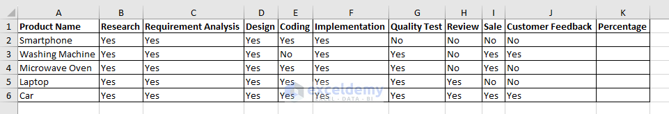
OUTPUT: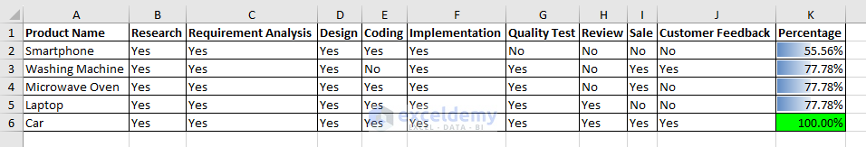
WORKBOOK: Data Bars And Conditional Formatting
Feel free to contact us again with any other inquiries or concerns.
Regards
Lutfor Rahman Shimanto
ExcelDemy
Dear ABDUL KADAR
Greetings from our website! Thank you for posting your question on the platform. As requested, I can assist you with an Excel formula using the IF and COUNTIFS functions that determine how many products a Region makes even if regardless of the product name (sometimes the product column is blank against a Region).
FORMULA:
Regards
Lutfor Rahman Shimanto
Hello CAR
Thank you for reaching out to us on our website. You can use a single module to move rows between sheets based on various values. You may do this by using an IF statement inside a FOR loop that iterates through the rows in Sheet1, verifies the value, and then moves the entire row to the proper destination sheet based on the value. The intended code is given below.
Regards
Lutfor Rahman Shimanto
Hello Ruby,
Greetings from our website. You have encountered a warning message from the Microsoft Excel window. The error message “You’ve entered too few arguments for this function” means not providing enough arguments or inputs for a particular formula or function to work correctly. To resolve this error, check the formula or function you’re using and ensure you’ve provided all the required arguments.
This article explains how we can highlight cells with more than three duplicates. But, if you need help understanding this post, you can follow another article on the ExcelDemy website link given below.
How to Do Conditional Formatting in Excel [Ultimate Guide]
Later go through this article to better understand and highlight if there are more than three duplicates. Good luck.
Regards
Lutfor Rahman Shimanto
Hello PRACHI DABHADE
Greetings from our website! Thank you for posting your question on the platform. I can assist you with an Excel VBA code that creates new workbooks and allows you to specify names for those files. Furthermore, you can choose a location to store those files. Note that the user can cancel the folder selection dialogue. If they do, the code will end without making any new workbooks.
Download Workbook:
I am attaching the Workbook used to explore your issue. You can have it by clicking the link below.
https://www.exceldemy.com/wp-content/uploads/2023/03/PRACHI-DABHADE.xlsm
INPUT:
In the sheet named Sheet1, there is a list of names.
OUTPUT:
the desired workbooks are created utilizing the Excel VBA code mentioned below.
VBA CODE:
NOTE:
1) I am using the Application.FileDialog method, this code asks the user to choose a folder where the new workbooks will be saved. Then, it puts the path to the selected folder in the folderPath variable.
2) Using the folderPath variable and the Workbook’s name from the wbNames array, the code saves each new Workbook with its name in the chosen folder.
3) Lastly, remember to modify the VBA code when you want to work with the other ranges. Don’t hesitate to contact us if you face any other issues.
Regards
Lutfor Rahman Shimanto (ExcelDemy Team)
Hello Patrick,
Thank you for reaching out with your issue. You encountered a Run-time error. The “Run-time error ‘9’: Subscript out of range” error occurs because you did not modify the VBA code and forgot to insert the intended sheet name. You are misled somehow by the first step of the third method. The post says to go to the Insert tab and choose Headers and Footer from the Text group, and then execute the code mentioned in the third method; that’s all.
I can provide three Excel VBA codes to avoid the error you experienced unintentionally. All you need to do is choose the intended sheet as the active sheet and run a sub-procedure from the below list.
First Method: Insert Page Number in Footer Using Excel VBA
Second Method: VBA to Insert Total Page Number in Footer
Third Method: Insert Page Number in Selected Cell
Regards
Lutfor Rahman Shimanto (ExcelDemy Team)
Hello DYLAN,
Thank you for reaching out to us on our website. I understand that you have a value assigned to each member and are trying to split them into equal groups while ensuring each group’s total weight is within 1. Based on your requirements, I can assist you with this by applying an Excel VBA code.
The above VBA code splits a list of items into groups based on their assigned value and calculates the total weighted value for each unique group. It loops through each row of the worksheet, sets each item to a group based on the total weighted value of the group, and creates a new group if the current group's total weighted value plus the contemporary item's assigned value is greater than 1. The GetUniqueValues function calculates the unique groups and their total weighted values by using the Unique and SUMIFS functions to generate an array of unique values in column C and calculate the total weighted value for each group.
1) Inserting Required Values:
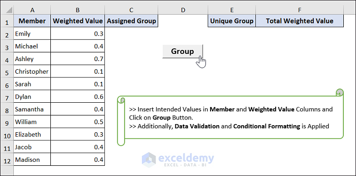
2) Displaying Final Output:
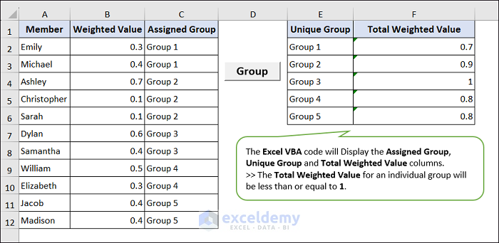
3) Download Practice Workbook
https://www.exceldemy.com/wp-content/uploads/2023/03/Dylans-Request.xlsm
Thank you again for reaching out to us, and I look forward to hearing from you soon.
Best regards,
Lutfor Rahman Shimanto
Hello KEVIN
Greetings from our website! Thank you for posting your question on the platform. I have yet to experience the issue you described personally. However, I can offer some insights to help you troubleshoot the problem.
The circular reference error may occur because the formula references the cell containing the procedure, creating an infinite loop. To avoid this, you can modify the system to refer to a different cell that doesn’t have the formula.
Excel’s built-in Error Checking feature can help identify and resolve circular references. To access this feature, go to the Formulas tab in the Excel ribbon, click Error Checking, and then click Circular References. Excel will then highlight any circular references in your workbook and suggest resolving them.
Providing any prominent solution without glancing at the workbook is challenging. You can share your workbook with us via Exceldemy Forum to better understand your situation.
Regards
Lutfor Rahman Shimanto (ExcelDemy Team)
Hello DAVID,
Thank you for reaching out with your comment. You encountered a different problem than what was described in the article. There could be several reasons why the problem is happening. Some of your add-ins may mess up the delete sheet feature, which may not work in your version of Microsoft Excel. To fix this, you should update your program.
You can use an Excel VBA code to delete a sheet by inputting the sheet name.
Excel VBA Code:
The VBA code and suggestions will solve your issue. Good luck.
Regards,
Lutfor Rahman Shimanto
Hello AYESHA
Thanks for your query. I have analyzed the workbook Rafiul Haq shared. A prominent approach to avoid data overlapping is to create the employee record separately for each month. So don’t hesitate to make the Employee Leave description for each month.
Regards
Lutfor Rahman Shimanto
Hello ERICH NAGY
I appreciate your time in reading the article. I’m delighted you found the information helpful and learnt something new. Your attention to detail is really appreciated, and you are correct. The appropriate range should be the C5:C20 range instead of D5:D20. An immediate correction will be made. Once again, We appreciate your comments and support. Continue reading our blog, and we aim to offer you further helpful information soon.
Regards
Lutfor Rahman Shimanto (ExcelDemy Team)
Hello ERIC SCHOENTHALER,
Thank you for your nice words! Great that you found our website and information helpful and relevant to your goal. I’m glad we could provide you with the information you were looking for. Regarding your question, you can use the following VBA code to insert a specific amount of page breaks starting at a particular line.
Regards
Lutfor Rahman Shimanto
Thank you so much for sharing this tip, Andy! I sincerely appreciate the time you took to share your expertise and assist others with this problem. Your suggestion proved effective, and We are genuinely grateful for it. Thank you again!
Regards
Lutfor Rahman Shimanto