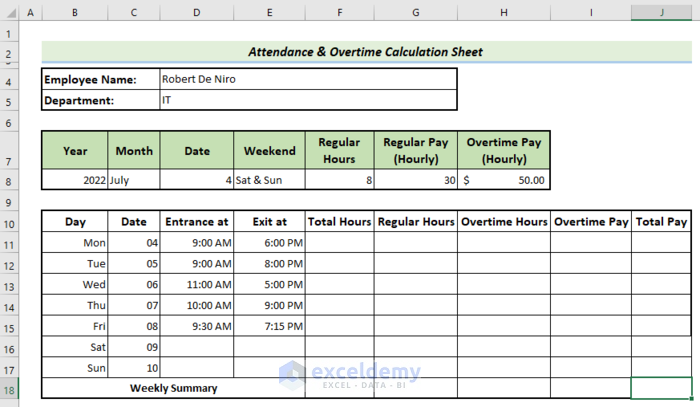
Attendance and Overtime Calculation Sheet in Excel

Step 1 – Set Year, Month, Date, and Weekend Data in a Helper Sheet

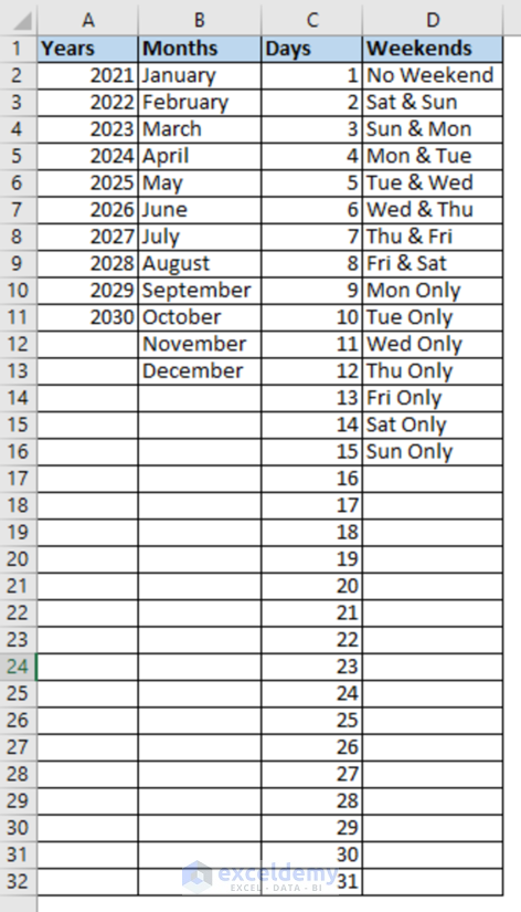
Make a dataset containing Years, Months, Days, and Weekends in a separate worksheet (named Data) as shown in the following image.

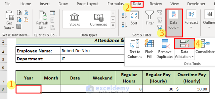
Select cell B8, then go to the Data tab, select Data Tools, and choose Data Validation.
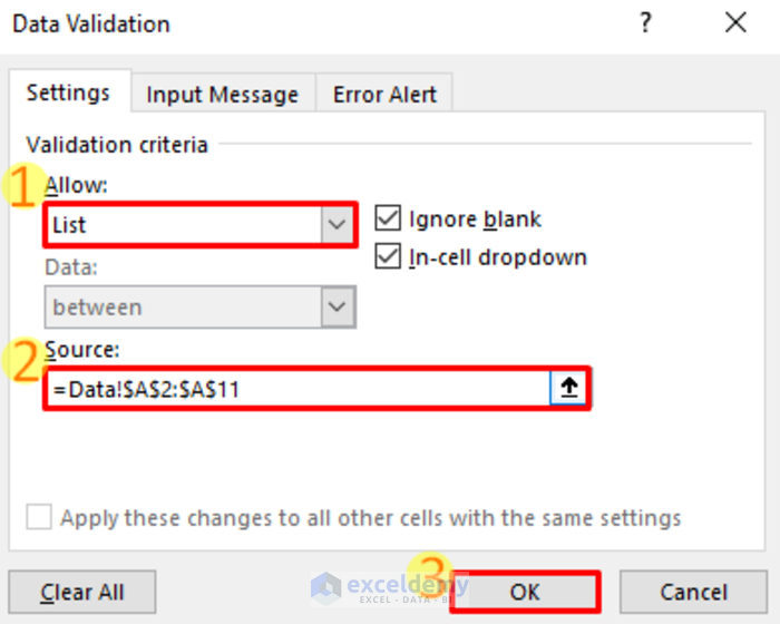
A Data Validation Window will pop up.

At the Allow box, choose List.
In the source box select the Year column from the sheet named Data (A2:A11).
Click on OK.

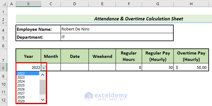
You will get a drop list of years.
Repeat the process to create drop-down lists for Month, Date, and Weekend. Every time you do, choose their respective data from the source sheet called Data.

Step 2 – Set the Dates in the Main Calculation Sheet

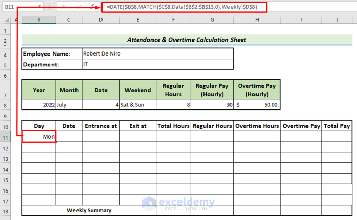
Use the following formula in B11.

=DATE($B$8,MATCH($C$8,Data!$B$2:$B$13,0),Weekly!$D$8)

Press Enter.

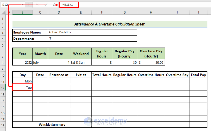
Put =B11+1 into cell B12, then press Enter.
Drag the Fill Handle down from B12 to the end of the column.

You can set the Date column by applying the following formula to cell C11, then pressing Enter.

=DATE($B$8,MATCH($C$8,Data!$B$2:$B$13,0),Weekly!$D$8)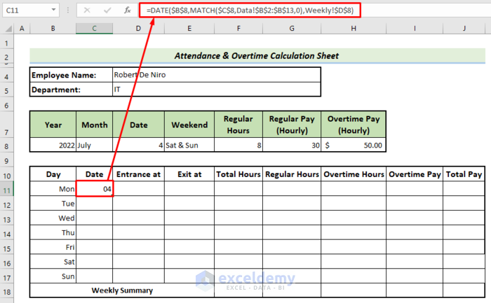

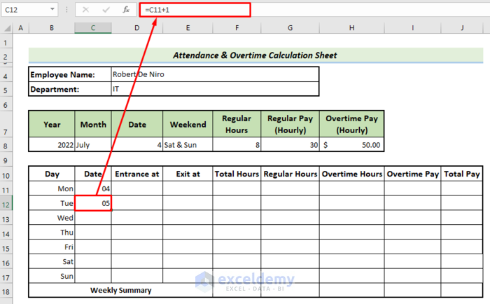
In cell C12, put =C11+1 to get the consecutive dates.
Drag down the formula to the rest of the cells.

Note:

You can specify the weekend. Drop-down menus offer a variety of options. You can choose no weekend, a 1-day weekend (Mon, Tue…), or a 2-day weekend (Fri & Sat, Sat & Sun..).

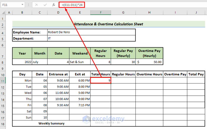
Step 3 – Calculate the Total Working Hours

Input the data for the Entrance and Exit columns for working days.
Inbuilt checks ensure ‘Entrance at’ isn’t later than ‘Exit at’. In such a scenario, the user would not be able to enter the time.

Calculate the total working hours in cell F11 using the following formula.

=(E11-D11)*24

Drag down the Fill handle to get the total working hours for the rest of the weekdays.

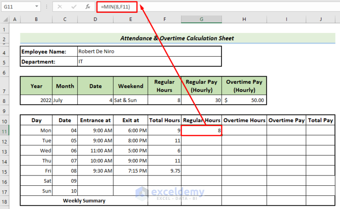
Step 4 – Set the Regular Office Hours and Calculate Overtime Hours

Use the following formula in cell G11.

=MIN(8,F11)

Here the MIN function results in the smaller value between 8 and total hours.

Use the following formula in cell H11 to get the overtime hours.

=(F11-G11)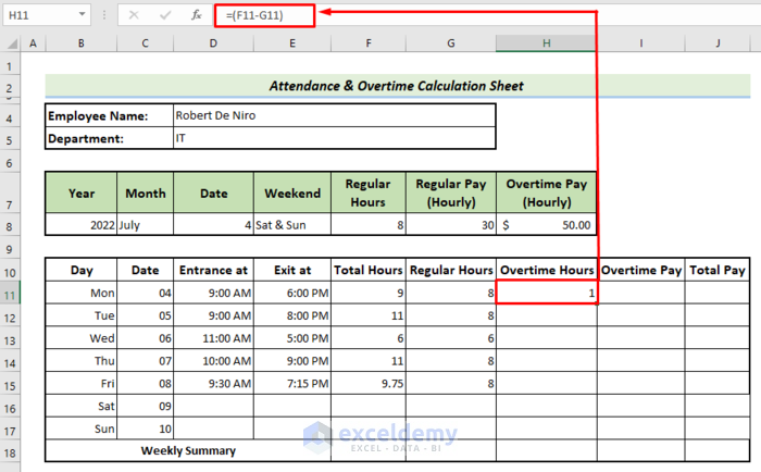

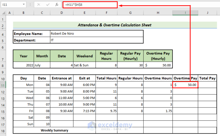
Step 5 – Calculate Overtime Pay

Use the following formula in I11:

=H11*$H$8

Here H8 contains the value of overtime pay hourly. If we multiply this value with overtime hours, it will return the overtime pay.

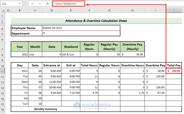
Step 6 – Calculate the Total Pay

In Cell J11, use the following formula to get the Total Pay.

=(G11*$G$8)+I11

(G11*$G$8) calculates regular pay, while I11 denotes overtime pay. The total pay is the sum of these two.

Step 7 – Make a Weekly Summary

AutoFill all the formulas from F11:J11 down.
Use the following formula in cell J18.

=SUM(J11:J17)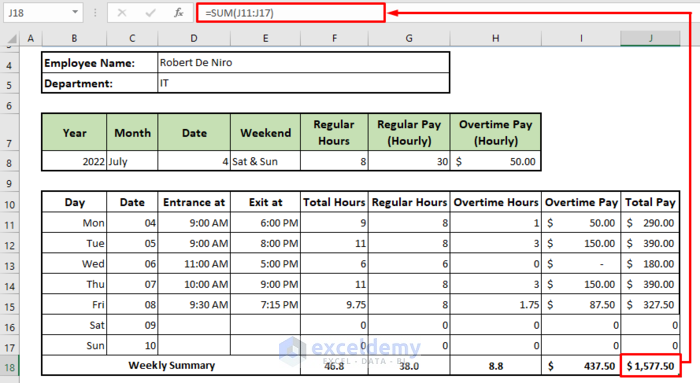

Download the Sample Workbook

Attendance and Overtime Sheet.xlsx

<< Go Back to Employee Attendance Sheet Excel | Excel HR Templates | Excel Templates

Get FREE Advanced Excel Exercises with Solutions!

4 Comments

Santosh Kumar Oct 26, 2023 at 12:22 PM

what if employee works for more than 24 hours regularly or 48 hours regularly, can we maintain calculation in single step or if it will be an exception
- Reply
  Joyanta Mitra Oct 26, 2023 at 3:35 PM
  
  Dear Santosh Kumar,
  Please clarify the question. How can a person do more than 24 hours in 24 hours?
  With Regards.
  Joyanta Mitra
g Dec 30, 2023 at 3:01 PM

I have an issue with the time, i entered different time and stated on excel different times. I can only do am and not pm. Could you assist?
- Reply
  Yousuf Khan Jan 15, 2024 at 11:53 AM
  
  Hello G,
  
  Thank you for sharing your experience with us! I understand you are facing time issues with your attendance & overtime calculations. You mentioned that you could only get AM time but not PM. This is interesting because Excel has no built-in time format that shows only AM and not PM. All standard time formats like h:mm AM/PM, hh:mm AM/PM, and m:ss AM/PM display both AM and PM for times before and after noon, respectively.
  
  The reason you are facing this issue could be your regional settings might be set to a locale that uses a 24-hour clock instead of a 12-hour clock with AM/PM indicators. To check your regional format and adjust your settings:
  1. Go to Control Panel.
  2. Click Clock and Region to see your existing time format.
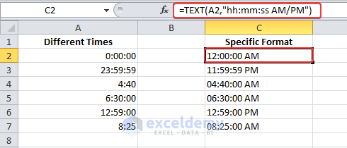
  Another reason could be a Custom Format has been applied to the cells that only show AM and hides PM. Whatever the reasons are, you can make it right using the specific time format. Follow the steps:
  1. Select a blank cell where you want the output.
  2. Enter the following TEXT formula and press Enter.
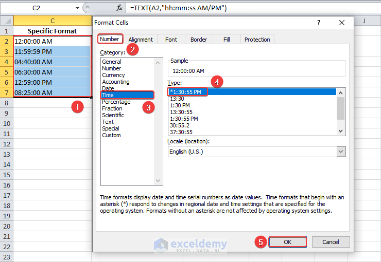
  =TEXT(A2,"hh:mm:ss AM/PM")
  
  As a result, the TEXT function converts different time values into text strings. If you want to calculate these times later, then set a custom format:
  1. Select the target cells and press Ctrl + 1.
  2. In the Format Cells dialog, click Time under Category.
  3. Select the desired format code in the Type box and click OK.
  
  Thus, you embed the desired time formats.
  
  Regards,
  Yousuf Shovon