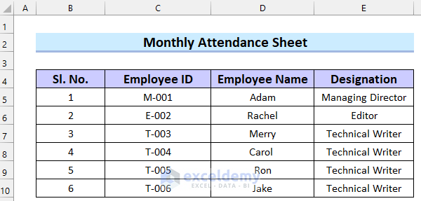
How to Create a Monthly Staff Attendance Sheet in Excel (With Easy Steps)

This dataset contains information about employees. Using this dataset, we will create a monthly staff attendance sheet in Excel in 7 easy steps.

Step 1: Creating a Monthly Menu

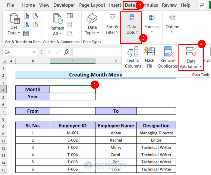
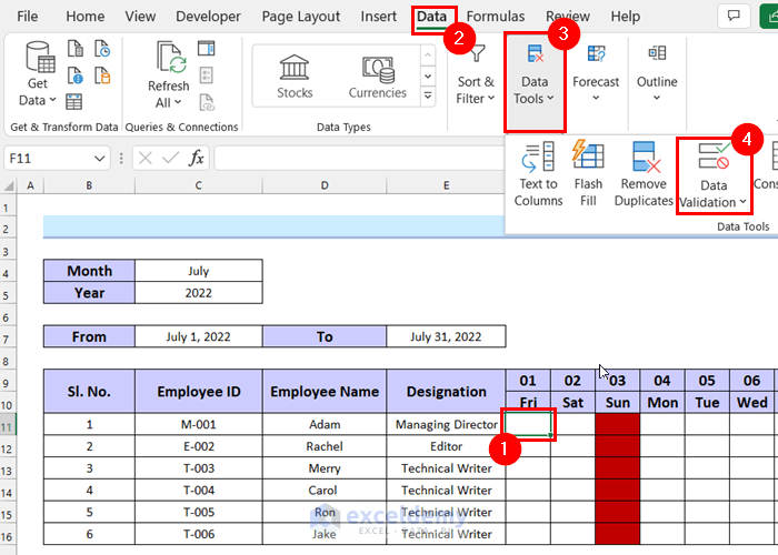
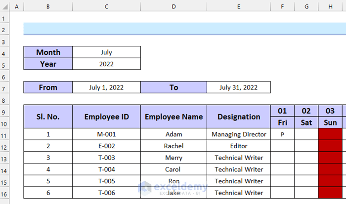
Select the cell where you want your month to appear. Here, I selected cell C4.
Go to the Data tab.
Select Data Tools.

Now, you will see a drop-down menu.

Select Data Validation from the drop-down menu.

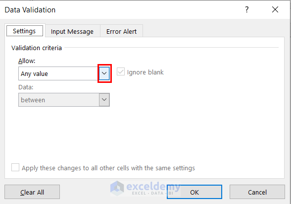
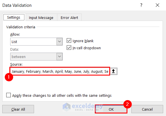
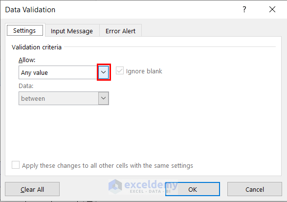
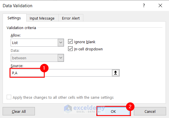
You will see a dialog box named Data Validation.

Select the drop-down option for Allow.

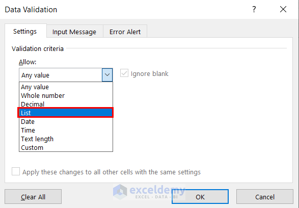
Select List from the drop-down menu.

Enter all the twelve months’ names as the Source.
Select OK.

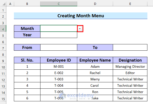
You will see that you have got a drop-down option for selecting a month in your Excel sheet.

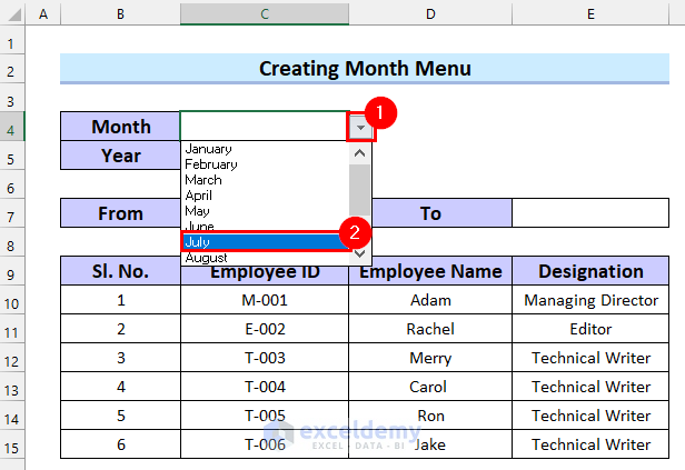
Click on the drop-down option.
Select your month. Here, I selected July.

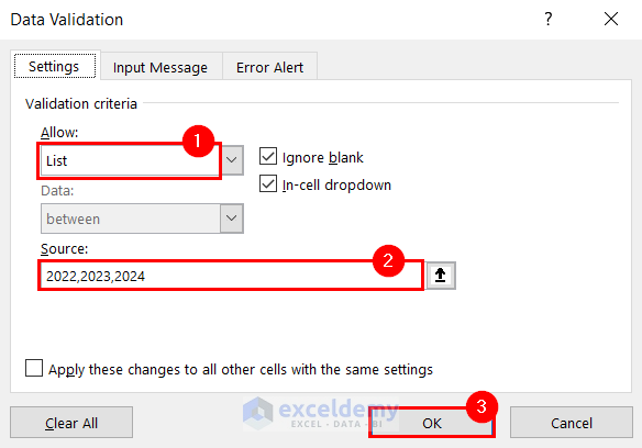
Following the previous steps, open the Data Validation dialog box to select the year.

Select List as Allow.
Eneer the years as the Source.
Select OK.

You will see that you have a drop-down option for selecting the year in your Excel sheet.

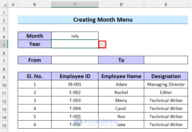
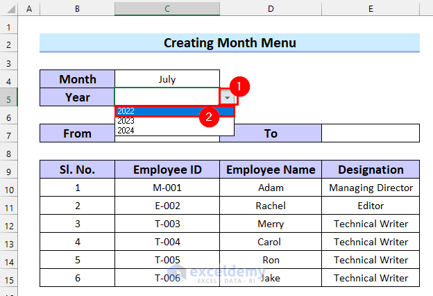
Click on the drop-down option.
Select your year. Here, I selected 2022.

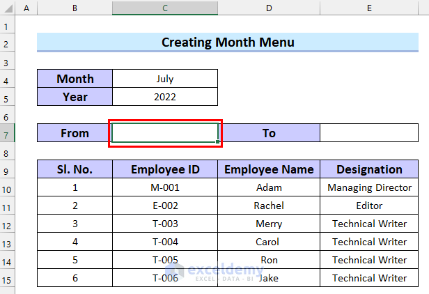
We will define the first and last date of the month.

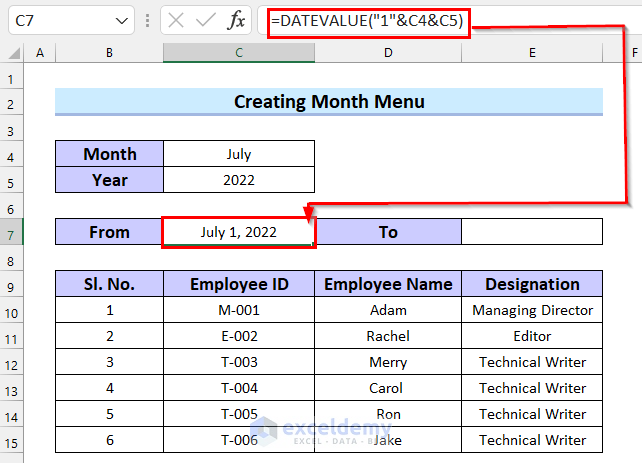
Select the cell where you want your first day of the month. Here, I selected cell C7.

In cell C7, enter the following formula:

=DATEVALUE("1"&C4&C5)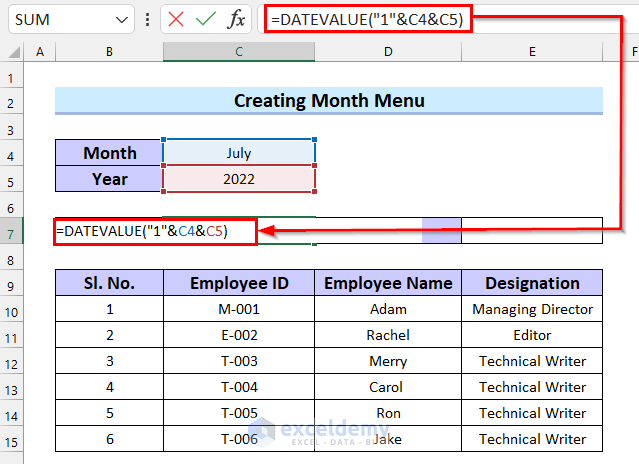

Here, I selected “1”, C4, and C5 as date_text in the DATEVALUE function. The formula will return on the first day of our selected month and year.

Press ENTER, and you will get your Date.

Select the cell where you want your last day of the month. Here, I selected cell E7.
In cell E7, enter the following formula:

=EOMONTH(C7,0)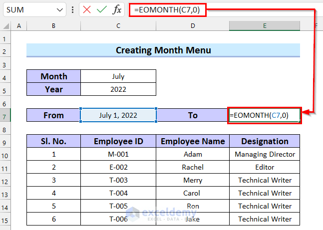

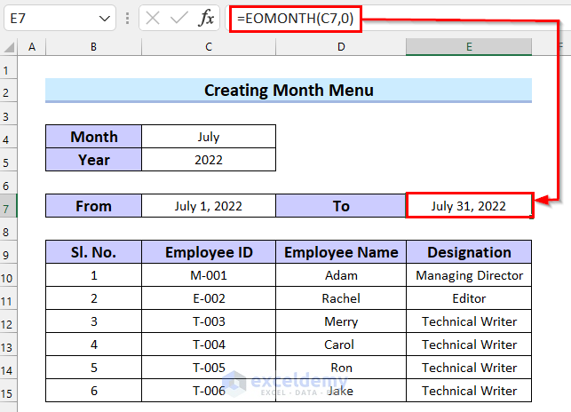
Here, in the EOMONTH function, I selected C7 as start_date and 0 as months. The function will return the last day of the current month.

Press ENTER.

Step 2: Inserting Dates into the Monthly Staff Attendance Sheet in Excel

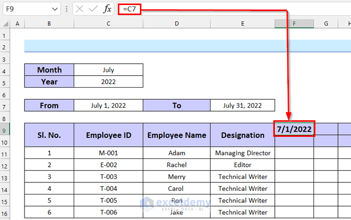
Select the cell where you want the first date. Here, I selected cell F9.
In cell F9, enter the following formula:

=C7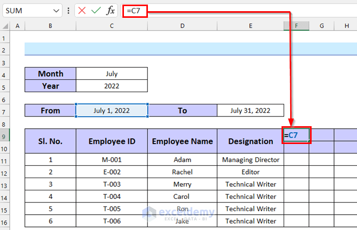

Here, I selected the value in cell C7 as the value in cell F9, which is the first day of the month.

Press ENTER, and you will get your date.

We will change to format of the date.

Right-click on the date.
Select Format Cells.

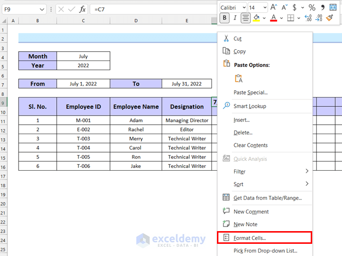
Here, the Format Cells dialog box will appear.

Select Custom.
Enter the custom format Type you want.
Select OK.

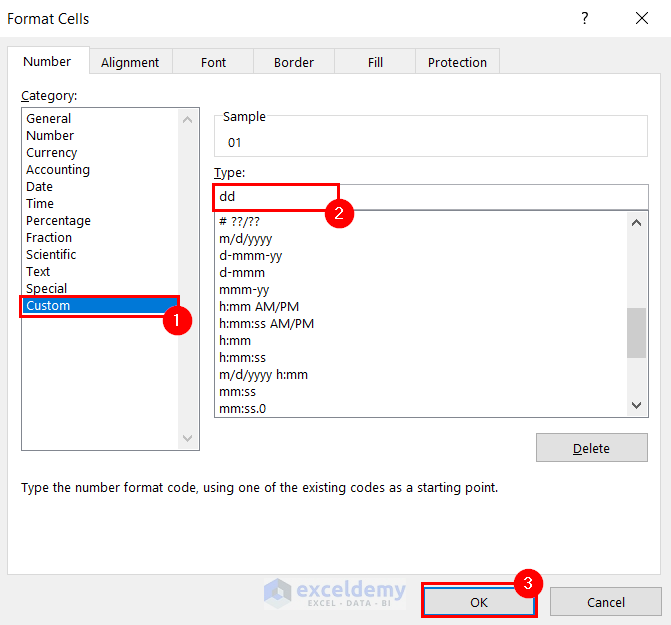
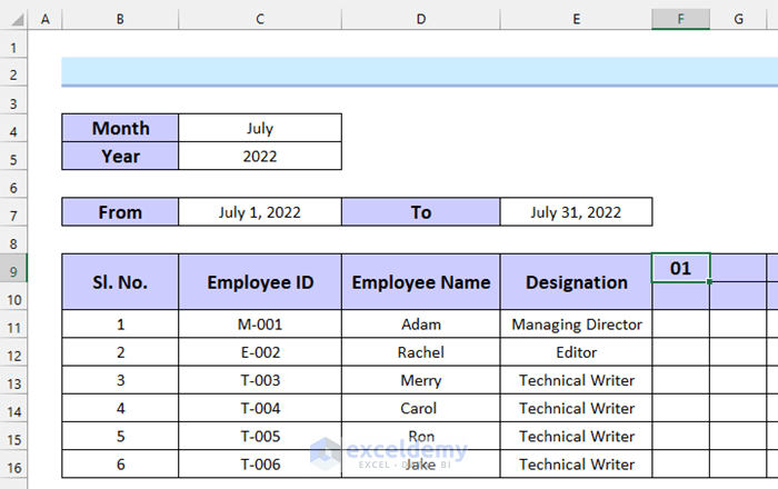
Now, you can see the desired format.

Select the next cell.
Enter the following formula:

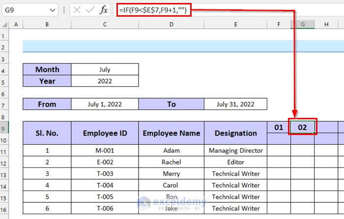
=IF(F9<$E$7,F9+1,"")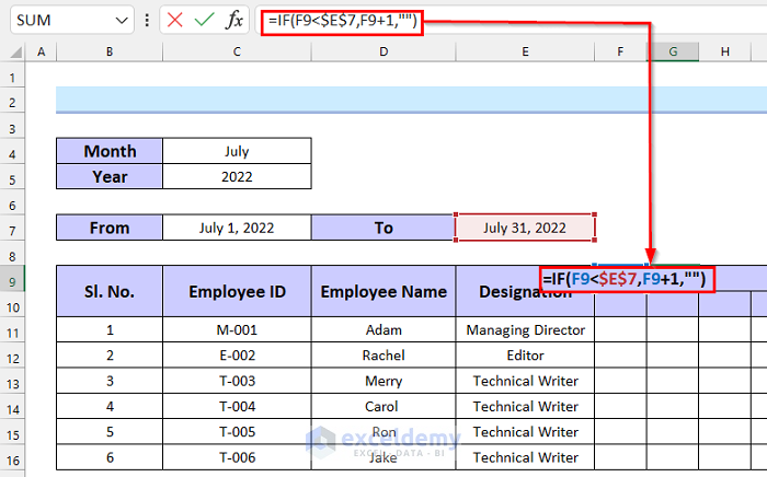

Here, in the IF function, I selected F9<$E$7 as logical_test, F9+1 as value_if_true, and blank as value_if_false. This formula will return the next date until it reaches the last date of the month.

Press ENTER to get the result.

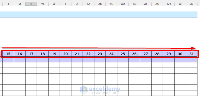
Drag the Fill Handle to copy the formula.

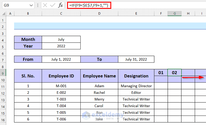
You can see that I have copied the formula.

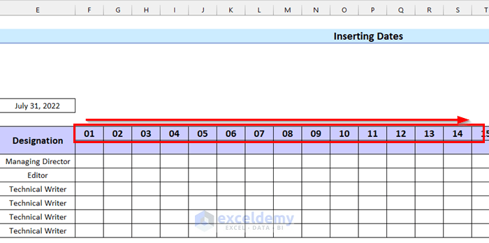
I copied it unitl I reached the last date of my month.

Step 3: Inserting Weekdays into the Monthly Staff Attendance Sheet in Excel

Select the cell where you want your first weekday of the month. Here, I selected cell F10.
In cell F10, enter the following formula.

=TEXT(F9,"ddd")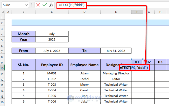

Here, in the TEXT function, I selected F9 as value and “ddd” as format_text. The formula will return the value in cell F9 in the given format.

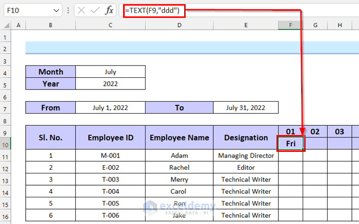
Press ENTER, and you will get your weekday.

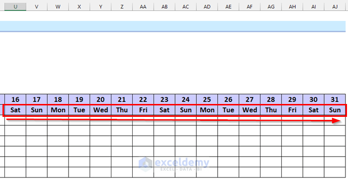
Drag the Fill Handle to copy the formula.

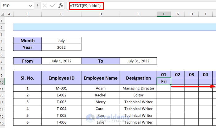
Here, you can see that I have copied the formula.

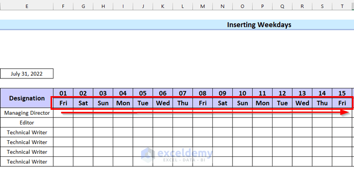
I copied it till I reached the last date of the month.

Step 4: Highlighting Weekly Holidays in the Monthly Staff Attendance Sheet in Excel

Select the first cell from where you want to highlight the holidays.
Go to the Home tab.
Select Conditional Formatting.

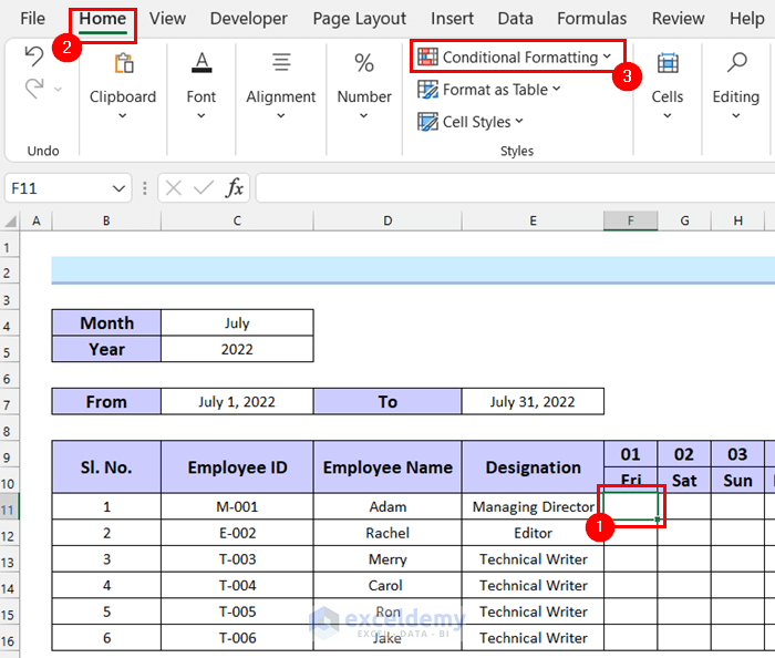
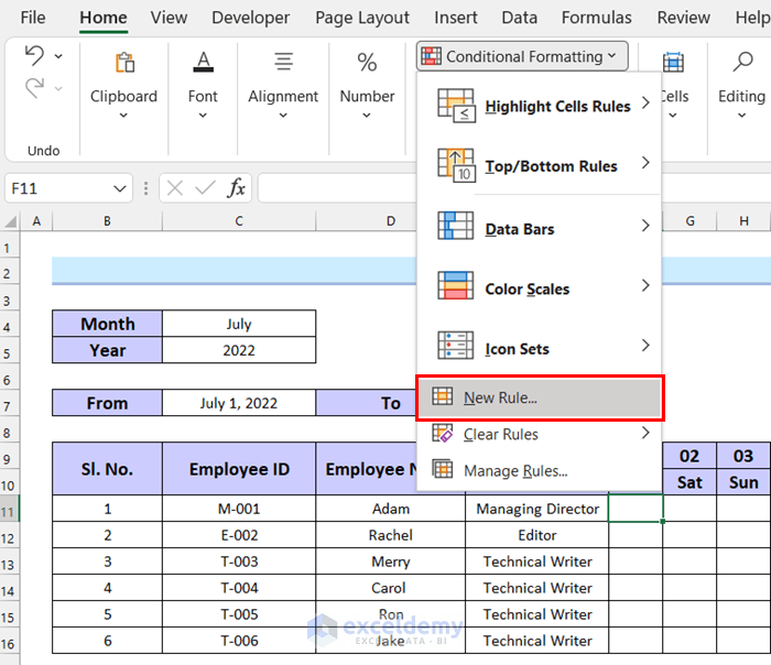
A drop-down menu will appear.

Select New Rule.

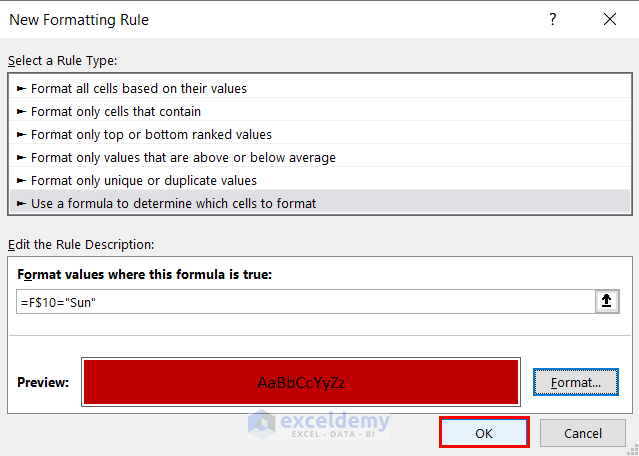
A dialog box named New Formatting Rule will appear.

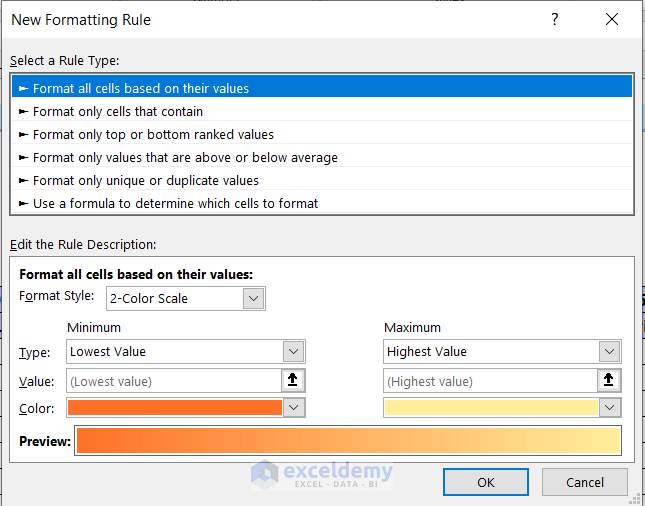
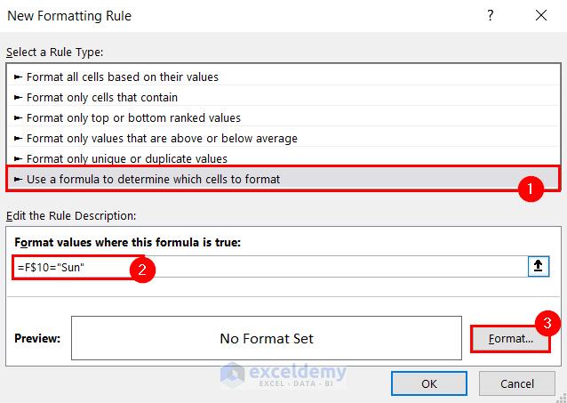
Select Use a formula to determine which cells to format.
Enter the formula for Format values where this formula is true. Here, I wrote the following formula:

=F$10=”Sun”

The formula will check Row 10 for the value “Sun” and format cells if the value is true.

Select Format.

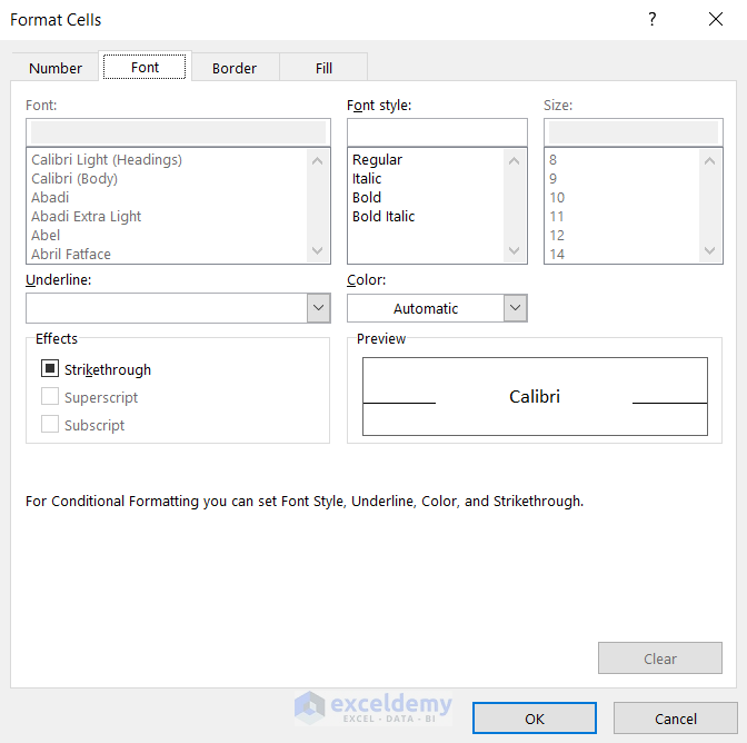
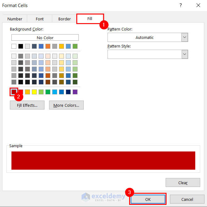
The Format Cells dialog box will appear.

Go to the Fill tab.
Select the color you want.
Select OK.

Here, the format will be added to the New Formatting Rule dialog box.

Select OK.

At this point, you will not see any change yet.

Select the cell you selected before.
Select Format Painter.

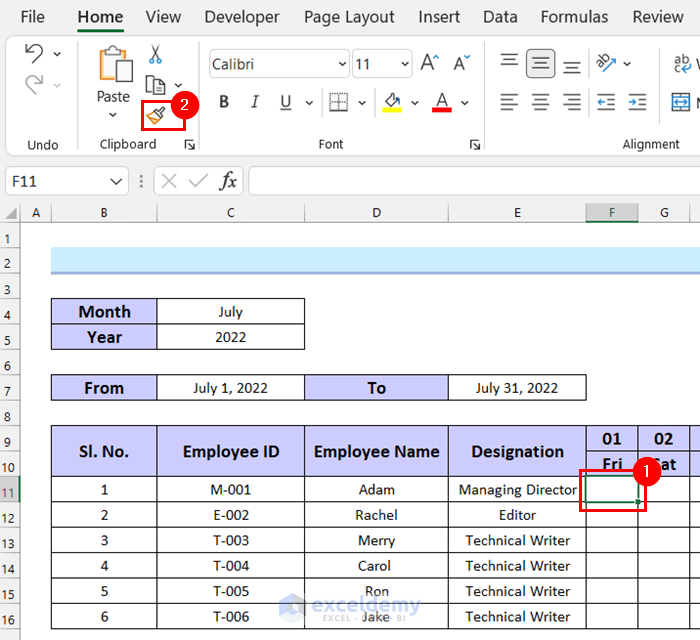
Drag the Fill handle and apply the formatting to your entire dataset.

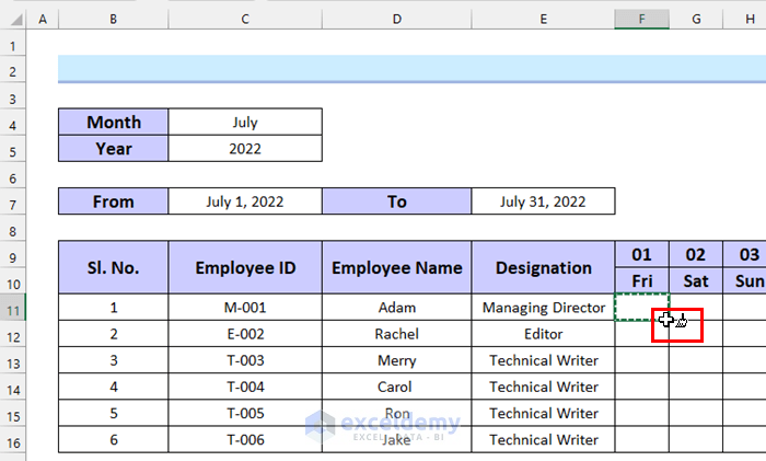
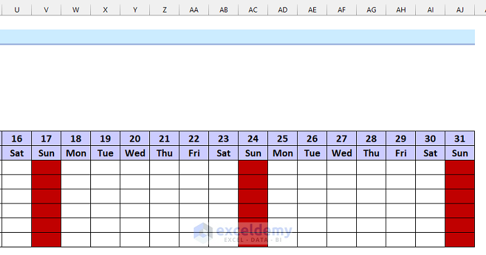
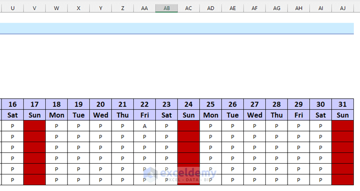
Here, you can see that I have applied the formatting to my entire dataset.

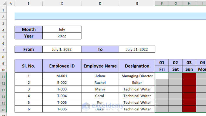
You can see that I have highlighted the weekly holidays in my monthly staff attendance sheet.

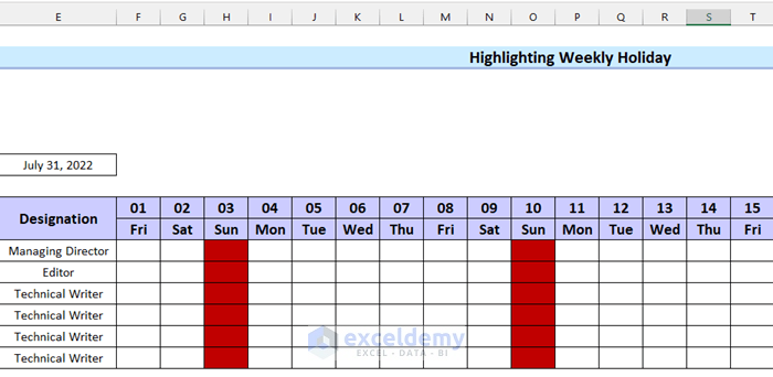
I have highlighted all Sundays throughout the month.

Step 5: Creating Input Attendance in Monthly Staff Attendance Sheet in Excel

Select the cell where you want your input attendance.
Go to the Data tab.
Select Data Tools.

You will see a drop-down menu.

Select Data Validation from the drop-down menu.

A dialog box named Data Validation will appear.

Select the drop-down option for Allow.

Select List from the drop-down menu.

Enter P and A as the Source. P stands for present, and A stands for absent.
Select OK.

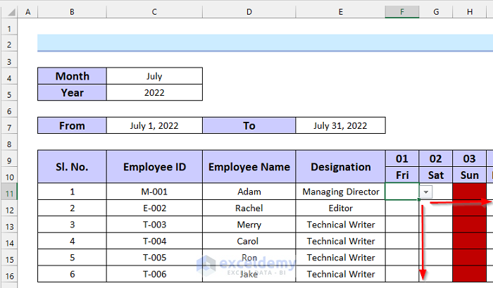
Now, you will see that you have a drop-down option for input attendance in your Excel sheet.

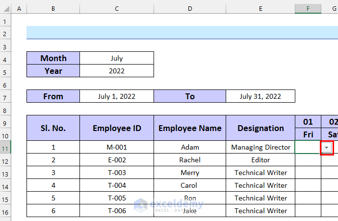
Drag the Fill Handle to copy this Data Validation throughout the attendance sheet.

Select the cell where you want your input attendance. Here, I selected cell F11.
Click on the drop-down option.
Select P if the person is present and A if the person is absent.

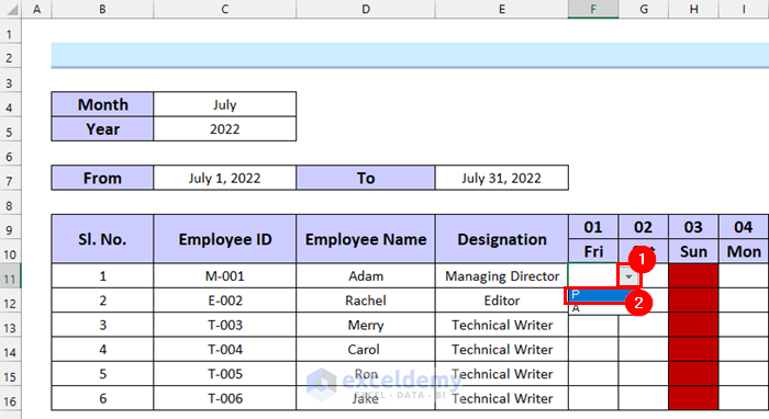
You can see I have input attendance for the employee named Adam for July 1, 2022.

Here, I filled out the whole attendance sheet.

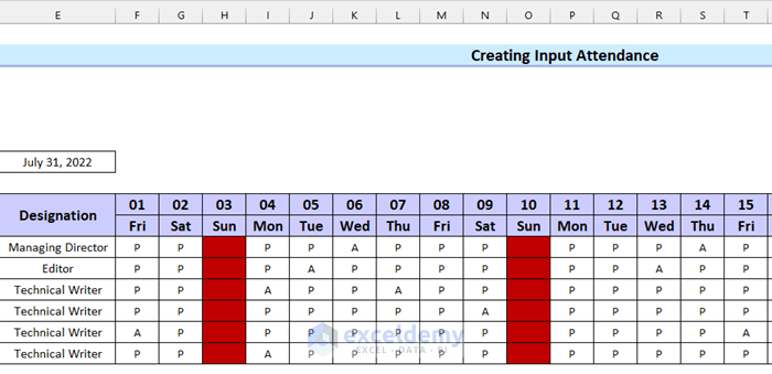
I filled it out until I reached the last date of my month.

Step 6: Counting Total Working Days

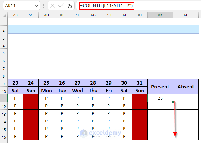
Select the cell where you want to count your total Present days. Here, I selected cell AK11.
In cell AK11, enter the following formula:

=COUNTIF(F11:AJ11,"P")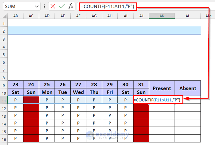

Here, in the COUNTIF function, I selected F11:AJ11 as the range and “P” as the criteria. The formula will count if the cells in the selected range contain “P”. It will return the total Present days.

Press ENTER to get the result.

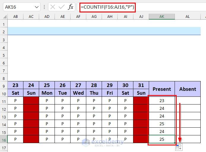
Drag the Fill Handle to copy the formula.

In the following picture, you can see that I have copied my formula for all the cells.

We will count the total Absent days.

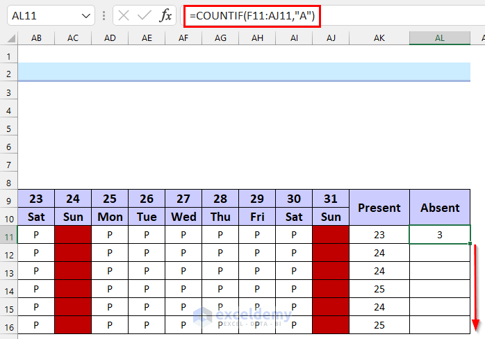
Select the cell where you want to count your total Absent days. Here, I selected cell AL11.
In cell AL11, enter the following formula:

=COUNTIF(F11:AJ11,"A")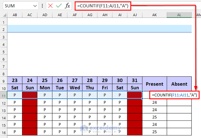

Here, in the COUNTIF function, I selected F11:AJ11 as the range and “A” as the criteria. The formula will count if the cells in the selected range contain “A”. It will return the total Absent days.

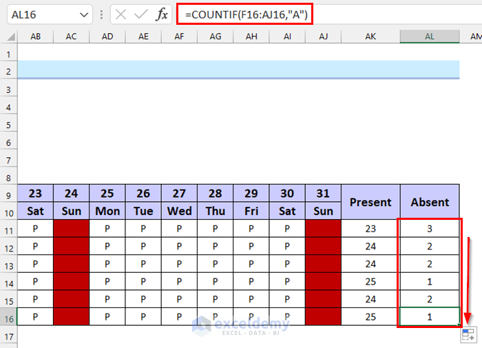
Press ENTER to get the result.

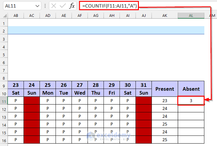
Drag the Fill Handle to copy the formula.

In the following picture, you can see that I have copied my formula for all the cells.

Step 7: Saving the Excel File as a Template

Go to the File tab.

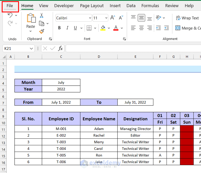
Select Save As.
Select Browse.

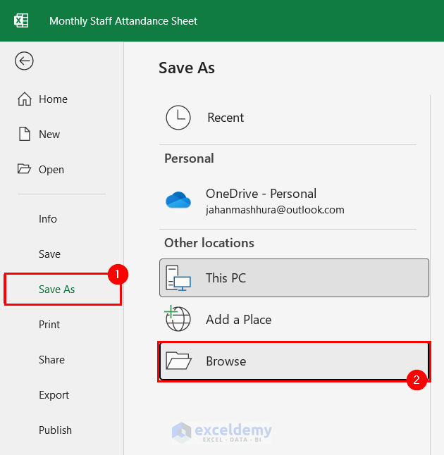
A dialog box named Save As will appear.

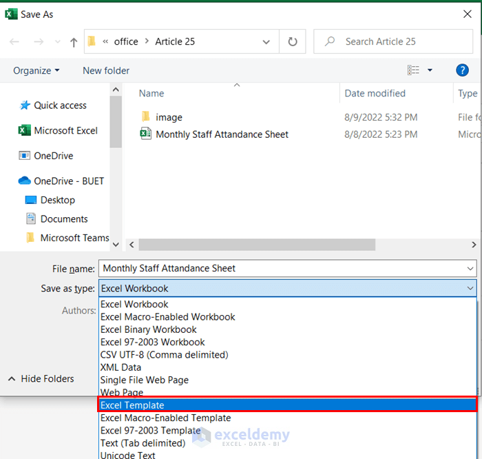
Select the drop-down option to select Save as type.

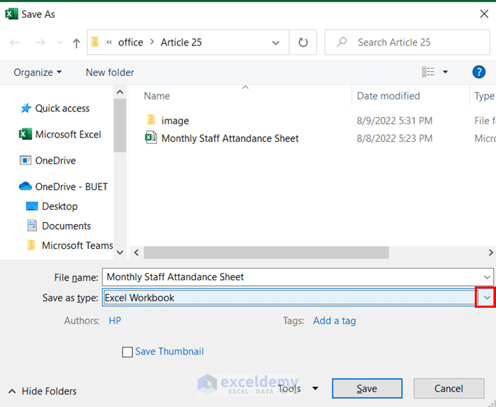
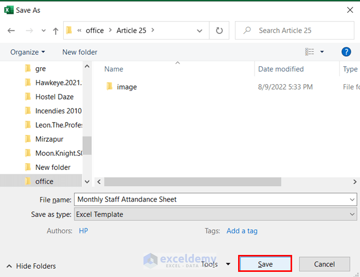
Select Excel Template from the drop-down menu.

Select Save.

Now, your file will be saved as a template, and you can access it while creating a new Excel file.

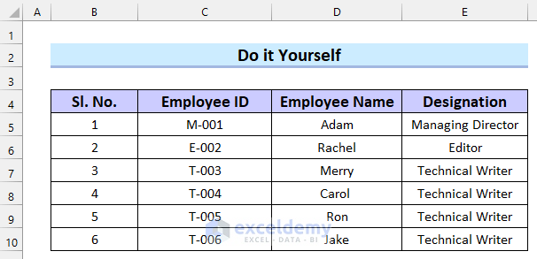
Practice Section

Here is a practice sheet for creating a monthly staff attendance sheet.

Download the Practice Workbook

Monthly Staff Attandance Sheet.xlsx

<< Go Back to Employee Attendance Sheet Excel | Excel HR Templates | Excel Templates

Get FREE Advanced Excel Exercises with Solutions!

6 Comments

siknader Aug 10, 2022 at 5:46 PM

unable to find datevalue for FEBURARY rest is working please do the needful.
- Reply
  Shamima Aug 21, 2022 at 2:48 PM
  
  Hi Sikander,
  Hope you are doing well.
  To get the DateValue for February, click on the drop-down option of Month and then select February.
  
  Then you will get the DateValue and the rest will be updated automatically.
  
  Note: If you want to type the month name in that cell you have to be careful with the spelling of the month name.
  
  Thanks
  
  Regards
  Shamima Sultana
Tudor Apr 19, 2023 at 9:22 PM

Hello, very well explained, but I have two questions:
1. How can I change the month and day from English to Romanian?
2. If an employee works on Saturday and/or Sunday, how can I collect those weekend hours separately, in a cell?
Thank You!
- Reply
  Shamima Sultana Apr 26, 2023 at 11:46 AM
  
  Dear Tudor,
  
  Hope you are doing well. Answer of your questions are given below with explanation.
  
  1. How can I change the month and day from English to Romanian?
  
  Select the cell with month and date, cell C7 in our case.
  Right-click with the mouse and select Format Cells.
  
  In the Format Cells window, select Romanian (Moldova) under the Locale menu.
  Then, select any type under the Type menu and click the OK button.
  
  The month and date are changed into Romanian from English. Do the same process for cell E7.
  
  2. If an employee works on Saturday and/or Sunday, how can I collect those weekend hours separately, in a cell?
  
  Let’s say the first employee works on Saturday and Sunday for 5 and 6 hours respectively. He works on 4 weekends which you can see in the picture. To sum these values we’ll use the SUMIFS function.
  Apply the formula in any cell where you want the weekend hours, let’s say cell AM11-
  =SUMIFS($F$11:$AJ$11,$F$11:$AJ$11,"<>P",$F$11:$AJ$11,"<>A")
  
  After pressing Enter you’ll get the total weekend hours. You can use the Fill Handle tool to apply this formula to other employees.
Ken Mambo Sep 15, 2024 at 4:41 PM

Thank you for this.
I want to request directions on adding a cumulative totals table of days present/absent month on month for the whole year.

Thank you.
- Reply
  Shamima Sultana Sep 16, 2024 at 1:02 PM
  
  Hello Ken Mambo,
  
  You are most welcome. To add a cumulative totals table for days present or absent using the article’s attendance sheet, you can follow these steps:
  
  Add a table with rows representing months and columns for each employee.
  In the cumulative table, for each month use:
  =COUNTIF(Range_of_Attendance, “P”) // For Present Days
  =COUNTIF(Range_of_Attendance, “A”) // For Absent Days
  
  For cumulative data, use:
  =SUM(January_Cell:Current_Month_Cell)
  
  This approach will give you cumulative totals month by month.
  
  Regards
  ExcelDemy