How to Create a Monthly Attendance Sheet in Excel Using Formula: 8 Steps

Step 1 – Creating a Month and Year Menu

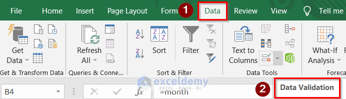
Go to any cell (i.e. C4) and insert the following formula:

=Month

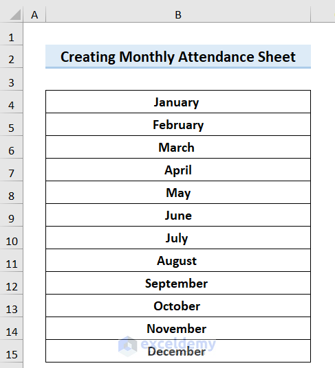
Open another sheet and enter all the months.

Return to the first worksheet and select the cell where you previously put the formula.
Go to the Data tab and select Data Validation.

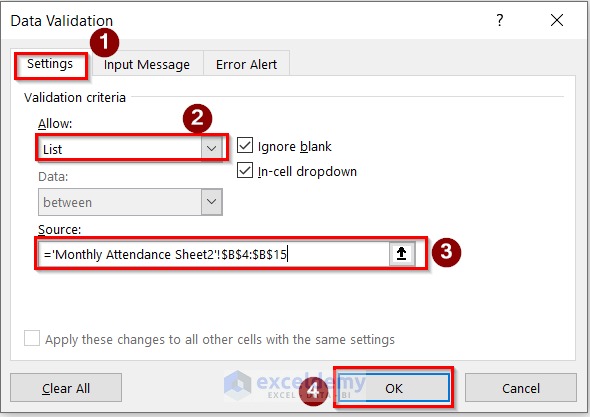
The Data Validation window opens.
Go to Settings and select List in the Allow tab.
Choose the list of the months in another worksheet in the Source option and press OK.

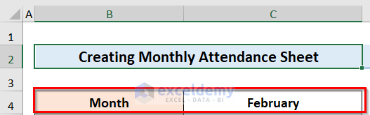
You will see the following result.

Select another blank cell(i.e. C5) and enter the following formula:

=year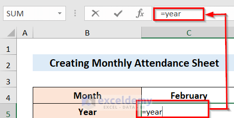

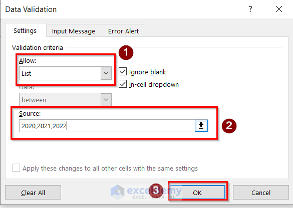
In the next cell, repeat the same steps that were performed for the month Select Cell > Data > Data Validation.

The Data Validation window opens. Enter 2020,2021,2022 in the Source and press OK.

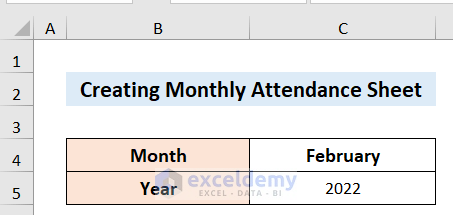
You will get a result similar to the following image.

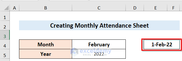
Step 2 – Inputting a Start and End Date of the Month

Go to any blank cell and insert the following formula:

=DATEVALUE( "1" &C4 &C5)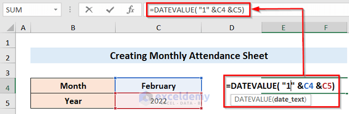

Press enter to find the below result.

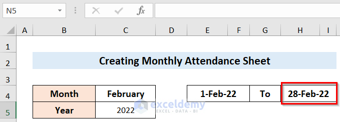
Go to another blank cell and insert the following formula:

=EOMONTH(E4,0)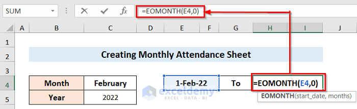

You will get a result similar to the following image.

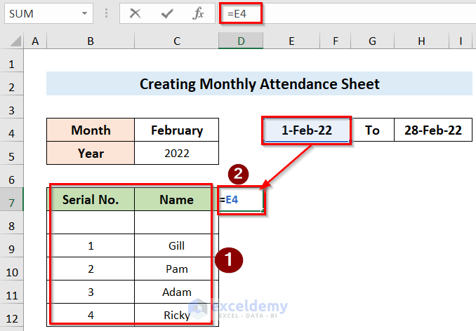
Step 3 – Inserting Dates Using IF Function.

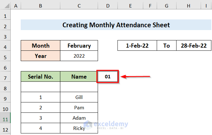
Enter the people’s names. (We have Serial No. in cell B7 and Name in cell C7).
Select any blank cell and refer to the starting date (in this case =E4) you created in the previous step.

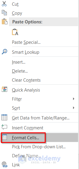
Right-click on the cell and select Format Cells.

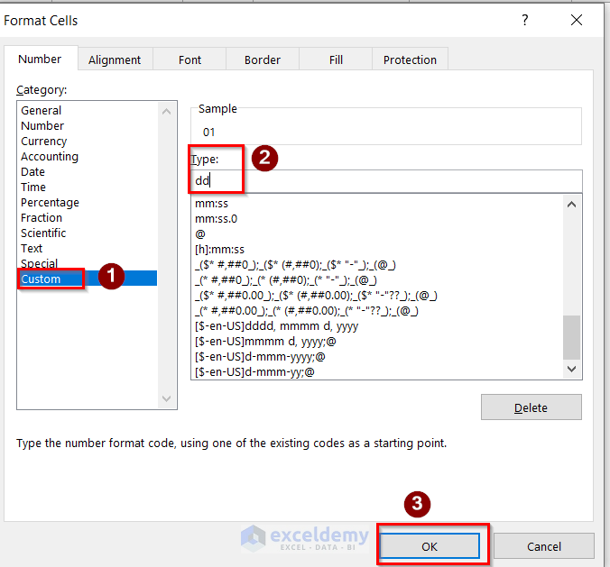
In the Format Cells window, go to Custom and type dd in the Type option. Press OK.

You will get the below result.

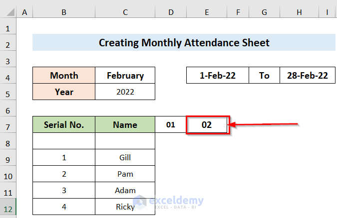
Select the blank cell next to the previous cell and insert the following formula:

=IF(D7<$H$4+1,D7+1,””)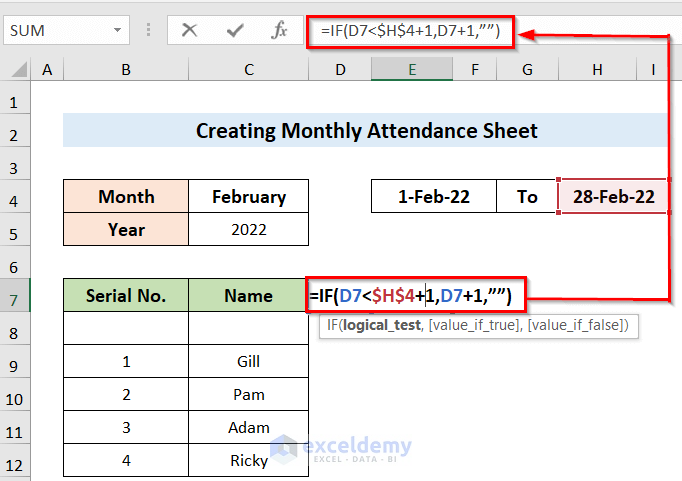

You will get this result.

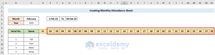
Use Fill Handle to fill in all the dates of the month.

Step 4 – Utilizing TEXT Function to Input Days

Select the cell below the first date (i.e. cell D7) and insert the following formula:

=TEXT(D7,"ddd")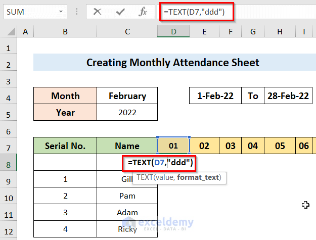

You will get the desired result.

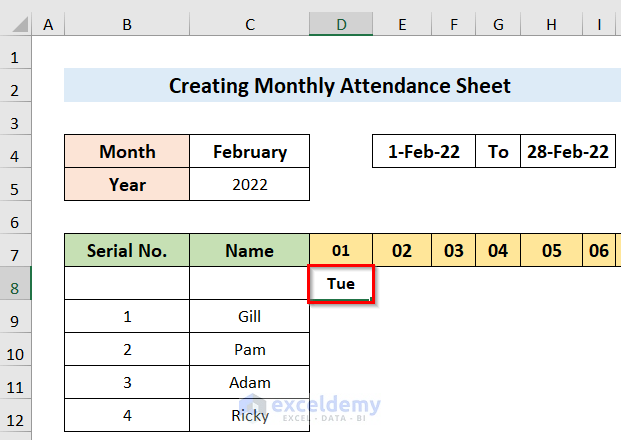
Use Fill Handle to get all the days of the month.

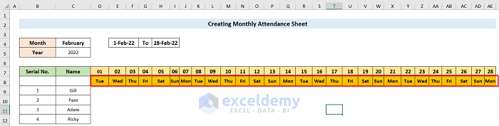
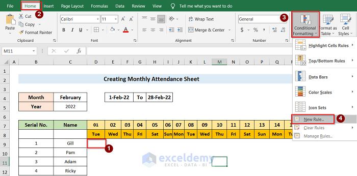
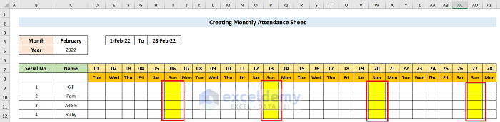
Step 5 – Highlighting Sundays in the Worksheet

Select the cell below the first day of the month and then go to the Home tab.
Go to Conditional Formatting and select the New Rule option.

In the New Formatting Rule window box, select the desired cell in the format value box:

=D$9="Sun"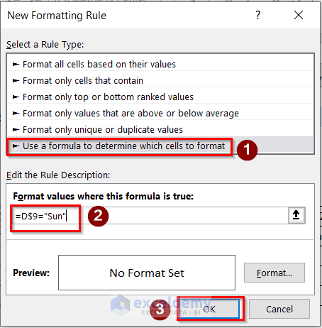

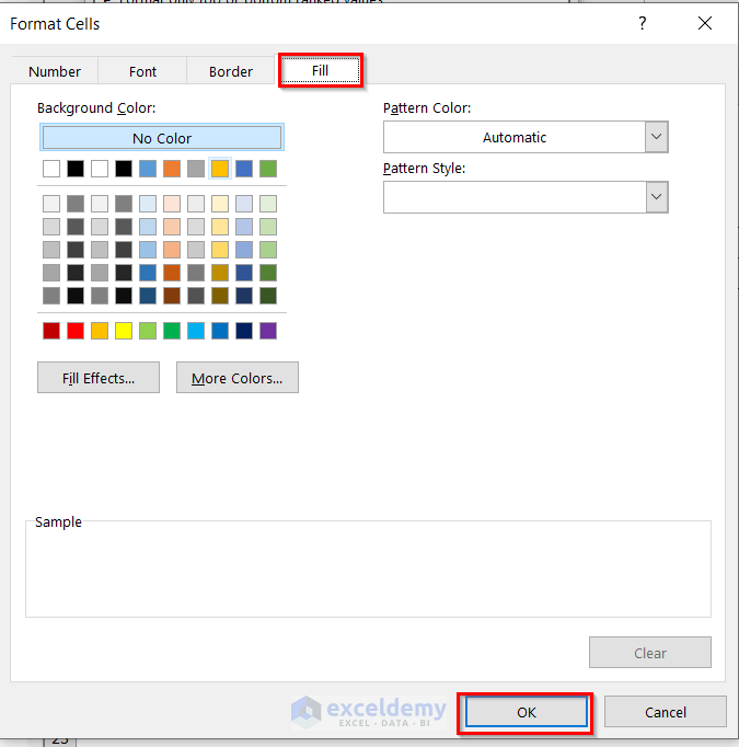
If you chose the Format option in the previous step, the Format Cells will appear on the screen.
Select the desired color from the Fill tab and press OK.

Select the cell you have used for the conditional formatting.
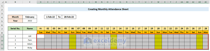
Select the Format Painter option and use Fill Handle to select all the cells to which you want this condition to apply.

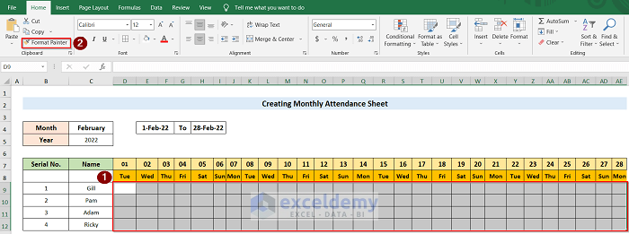
You will get results similar to the below image.

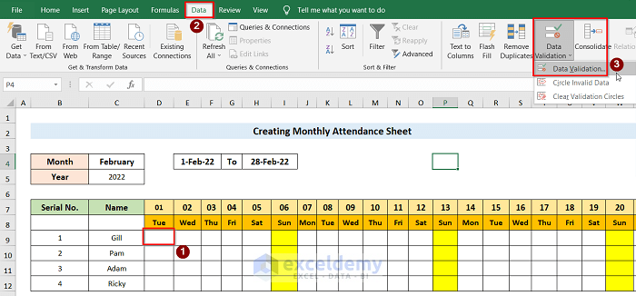
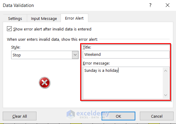
Step 6 – Restricting Data Entry on a Weekend

Select the first day of the month (i.e. cell D8) and choose Data Validation from the Data tab.

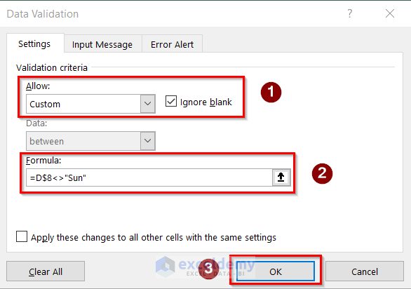
Select Custom in the Allow section.
Click Formula in the Setting tab under Data Validation.
Enter the following formula:

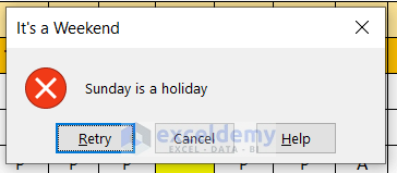
=D$8<>"Sun"

Press OK.

In the Error Alert tab, choose a Title and Error message and press OK.

Apply this to all desired cells using the Fill Handle.

You will get the below result.

Step 7 – Tracking Present and Absent Days

Enter the data of all names and create Present and Absent headings in two cells.

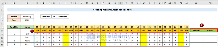
In the first cell under the Present heading, enter the following formula:

=COUNTIF(D9:AE9,"P")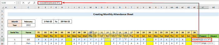

In the first cell under the Absent heading, insert the following formula:

=COUNTIF(D9:AE9,"A")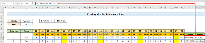

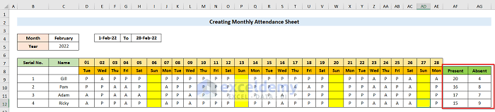
Use the Fill Handle to apply these formulas to the desired cells to get the below result.

Step 8 – Saving a Desired File as a Template

You want to save the whole datasheet as a Template file.
Choose the File option and press Save As. Save the file with the desired name.

Download the Practice Workbook

You can download the practice workbook from here.

Monthly Attendance Sheet.xlsx

<< Go Back to Employee Attendance Sheet Excel | Excel HR Templates | Excel Templates

Get FREE Advanced Excel Exercises with Solutions!

Private Sub Worksheet_Change(ByVal Target As Range) 'Developed by ExcelDemy If Target.Address = "$C$4" Or Target.Address = "$C$5" Then totalDays = Array(31, 28, 31, 30, 31, 30, 31, 31, 30, 31, 30, 31) If Range("C5").Value Mod 4 = 0 Then totalDays(1) = 29 End If Dim specificDate As Date Dim dayOfWeek As Integer Dim dayName As String monthNumber = Month(DateValue(Range("C4").Value & " 1 2000")) yearNumber = Range("C5").Value Range(Range("D7").Cells(1, 1), Range("D7").Cells(6, 31 + 2)).ClearContents Range(Range("D7").Cells(1, 29), Range("D7").Cells(6, 31 + 2)).ClearFormats For i = 1 To totalDays(monthNumber - 1) ' Specify the date specificDate = DateSerial(yearNumber, monthNumber, i) ' Get the day of the week as a number (1 for Sunday, 2 for Monday, etc.) dayOfWeek = Weekday(specificDate, vbSunday) ' Get the name of the day of the week dayName = WeekdayName(dayOfWeek, False, vbSunday) ' Display the name of the day Range("D7").Cells(1, i) = i Range("D8").Cells(1, i) = Left(dayName, 3) Next i Range("D7:D12").Copy For i = 29 To totalDays(monthNumber - 1) Range("D7:D12").Cells(1, i).PasteSpecial Paste:=xlPasteFormats Range("D7:D12").Cells(1, i).ColumnWidth = Range("D7").Cells(1, 1).ColumnWidth Next i Application.CutCopyMode = False Range("D7:D12").Cells(2, totalDays(monthNumber - 1) + 1) = "Present" Range("D7:D12").Cells(2, totalDays(monthNumber - 1) + 1).Interior.Color = vbGreen Range("D7:D12").Cells(2, totalDays(monthNumber - 1) + 1).ColumnWidth = 8 Range("D7:D12").Cells(2, totalDays(monthNumber - 1) + 1).Font.Bold = True Range("D7:D12").Cells(2, totalDays(monthNumber - 1) + 1).HorizontalAlignment = xlHAlignCenter Range("D7:D12").Cells(2, totalDays(monthNumber - 1) + 1).VerticalAlignment = xlVAlignCenter Range("D7:D12").Cells(2, totalDays(monthNumber - 1) + 2) = "Absent" Range("D7:D12").Cells(2, totalDays(monthNumber - 1) + 2).Interior.Color = vbGreen Range("D7:D12").Cells(2, totalDays(monthNumber - 1) + 2).ColumnWidth = 8 Range("D7:D12").Cells(2, totalDays(monthNumber - 1) + 2).Font.Bold = True Range("D7:D12").Cells(2, totalDays(monthNumber - 1) + 2).HorizontalAlignment = xlHAlignCenter Range("D7:D12").Cells(2, totalDays(monthNumber - 1) + 2).VerticalAlignment = xlVAlignCenter For j = 1 To 2 For k = 1 To 5 With Range("D7:D12").Cells(2, totalDays(monthNumber - 1) + 1).Cells(k, j) .Borders(xlEdgeTop).LineStyle = xlContinuous .Borders(xlEdgeTop).Color = RGB(0, 0, 0) .Borders(xlEdgeTop).Weight = xlThin .Borders(xlEdgeBottom).LineStyle = xlContinuous .Borders(xlEdgeBottom).Color = RGB(0, 0, 0) .Borders(xlEdgeBottom).Weight = xlThin .Borders(xlEdgeLeft).LineStyle = xlContinuous .Borders(xlEdgeLeft).Color = RGB(0, 0, 0) .Borders(xlEdgeLeft).Weight = xlThin .Borders(xlEdgeRight).LineStyle = xlContinuous .Borders(xlEdgeRight).Color = RGB(0, 0, 0) .Borders(xlEdgeRight).Weight = xlThin End With Next k Next j End If End Sub

2 Comments

Sam Jul 4, 2023 at 9:23 PM

I made this tracker, however, whenever I add ‘A’ or ‘P’ it doesn’t change with the month, it just stays in the specific cell.

Afia Kona Jul 10, 2023 at 10:21 AM

Dear Sam,
Thank you for your comment. I understand that you are looking for a more dynamic Attendance Sheet, if so, you can use the following VBA code as an update:

Download this Excel file for a better understanding.
I hope that your problem will be solved now. If you have any further issue, please let us know in the comment section.

Best
Afia Aziz Kona
Excel and VBA Content Developer
Exceldemy