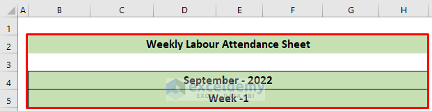
Step 1 – Prepare a Weekly Attendance Sheet Format
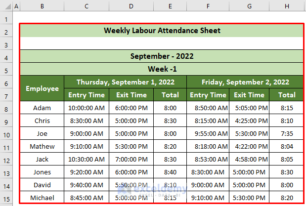
- Create some heading about the month and week number of your attendance Excel sheet in cells B4 and B5.
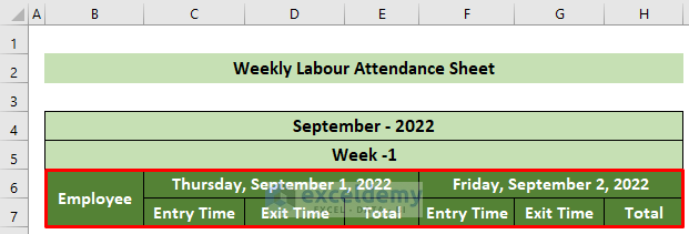
- In rows 6 and 7, create the headers for Employee names, dates, entry time, exit time, and total working time like in the image below.
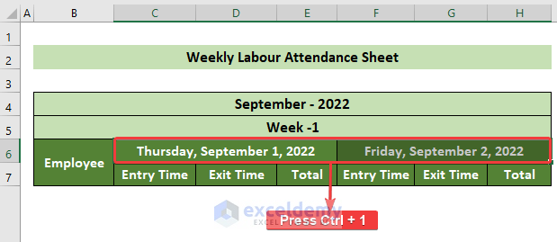
- Select merged cells C6 and F6.
- Press Ctrl + 1.
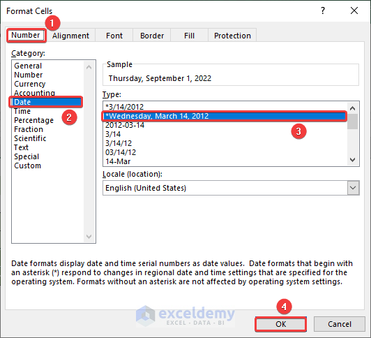
- The Format Cells window will appear.
- Go to the Number tab and choose Date from the Category pane.
- Select a date format that seems most legible for you and press OK.
- Select as many new rows below the headers as you have workers to manage (plus a few more if you plan to hire). C
- Select All Borders, Center, and Middle Align from the Font and Alignment subsections.
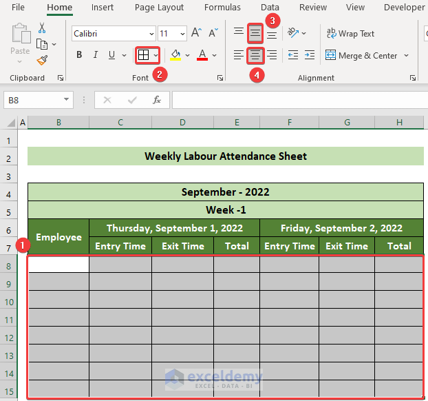
- Your labor attendance sheet in Excel format is ready to take inputs.
Read More: Attendance Sheet in Excel with Formula for Half Day
Step 2 – Record Entry and Exit Times
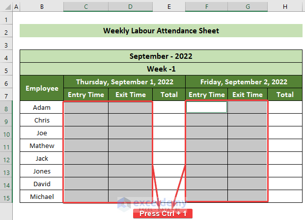
- Input the employees’ names in cells B8:B15.
- Select cells C8:C15, D8:D15, F8:F15, and G5:G18.
- Press Ctrl + 1.
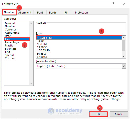
- The Format Cells window will appear.
- Go to the Number tab and choose Time from the Category list on the left.
- Choose the 1:30:55 PM option from the Type pane and click on the OK button.
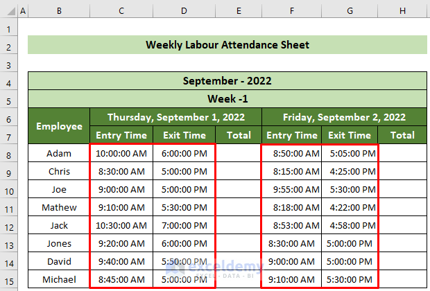
- Put the entry and exit times for all employees.
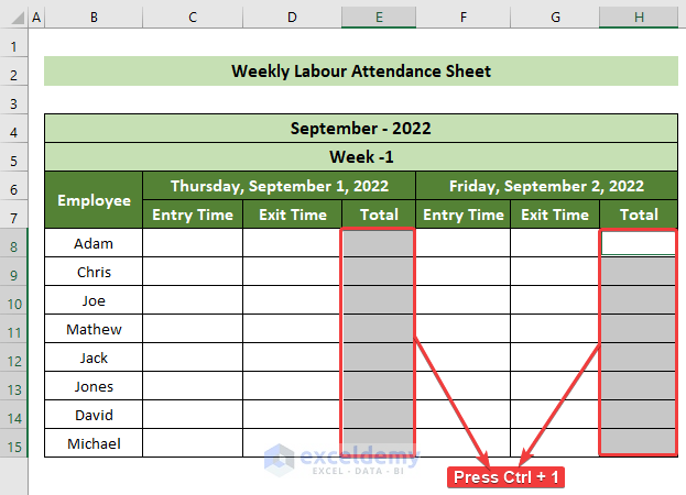
Step 3 – Calculate Total Time Worked
- Select cells E8:E15, and H8:H15.
- Press Ctrl + 1.
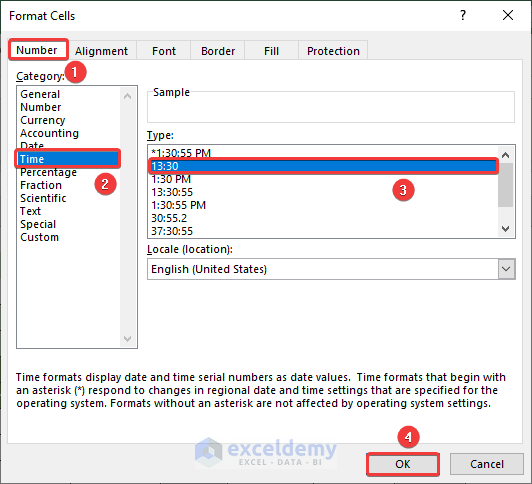
- The Format Cells window will appear.
- Go to the Number tab here and choose the Time option from the Category: pane.
- Choose the 13:30 option from the Type option list and click on the OK button.
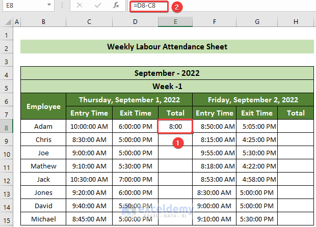
- Click on cell E8 and insert the following formula:
=D8-C8- Press Enter.
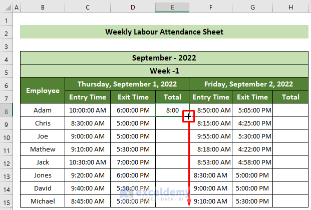
- Drag the Fill Handle down to fill in the other cells.
- Click on cell H8 and insert the following formula:
=G8-F8- Hit the Enter key.
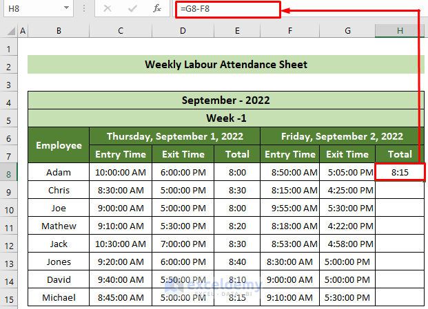
- Use the Fill Handle feature to get the employees’ total working time for that particular day.
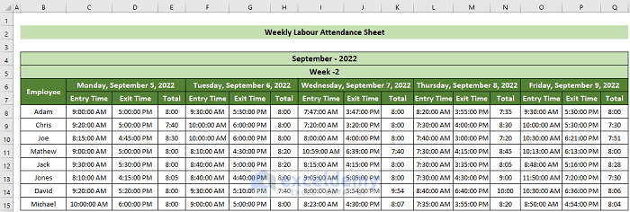
- Repeat for all the days and get all the weeks’ working time for all employees.
Read More: How to Create Employee Attendance Sheet with Time in Excel
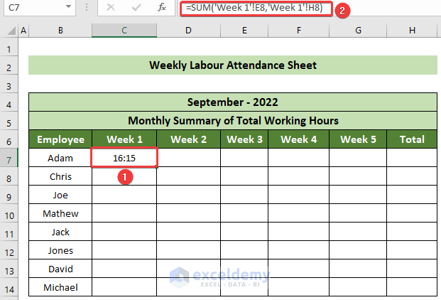
Step 4 – Prepare a Monthly Summary
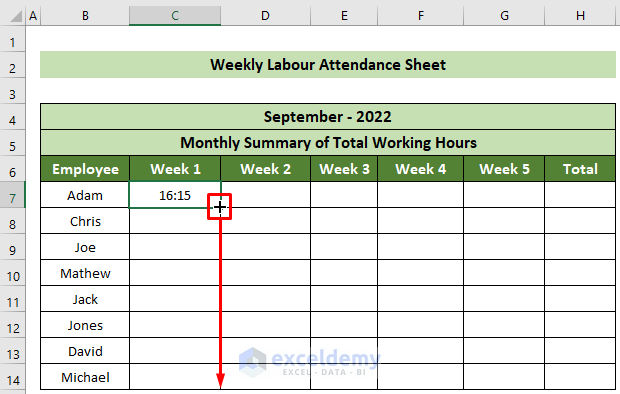
- Click on cell C7 and insert the following formula:
=SUM('Week 1'!E8,'Week 1'!H8)- Press the Enter key.
- Drag your Fill Handle down to copy the same formula for all the cells in the column.
- Click on cell D7 and insert the following formula for Week 2 total working hours:
=SUM('Week 2'!E8,'Week 2'!H8,'Week 2'!K8,'Week 2'!N8,'Week 2'!Q8)- Hit the Enter key.
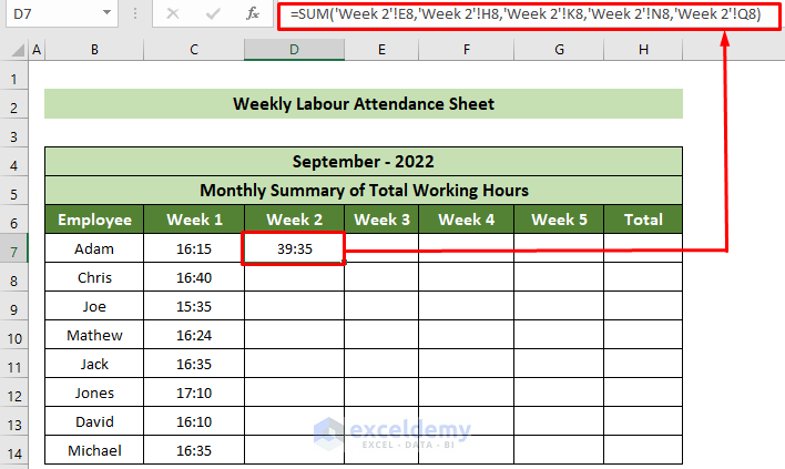
- AutoFill through the column via the Fill Handle.
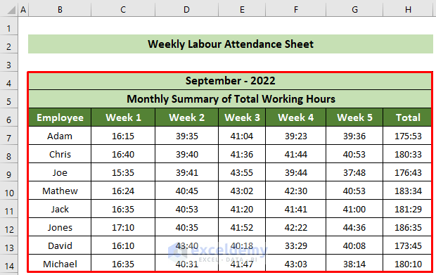
- Repeat the same procedures for other weeks, modifying the formula as needed.
Read More: How to Create a Monthly Staff Attendance Sheet in Excel
Download the Practice Workbook
You can download our practice workbook from here for free and use it as a template.
Related Articles
- How to Prepare a Meeting Attendance Sheet in Excel
- Attendance and Overtime Calculation Sheet in Excel
- How to Create Monthly Attendance Sheet in Excel with Formula
- How to Create Biometric Attendance Report in Excel
- How to Create Training Attendance Sheet in Excel
- How to Create Attendance Sheet with Time in and Out in Excel
<< Go Back to Employee Attendance Sheet Excel | Excel HR Templates | Excel Templates
Get FREE Advanced Excel Exercises with Solutions!
