In this tutorial, we will assume you have an attendance sheet of 10 workers for the month of January in 2022. You have a record of the holidays of the given month and the leaves taken by each employee. The resulting dataset looks like the image below:
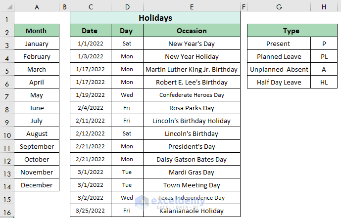
From here, the employees have taken both full day leaves and half day leaves.
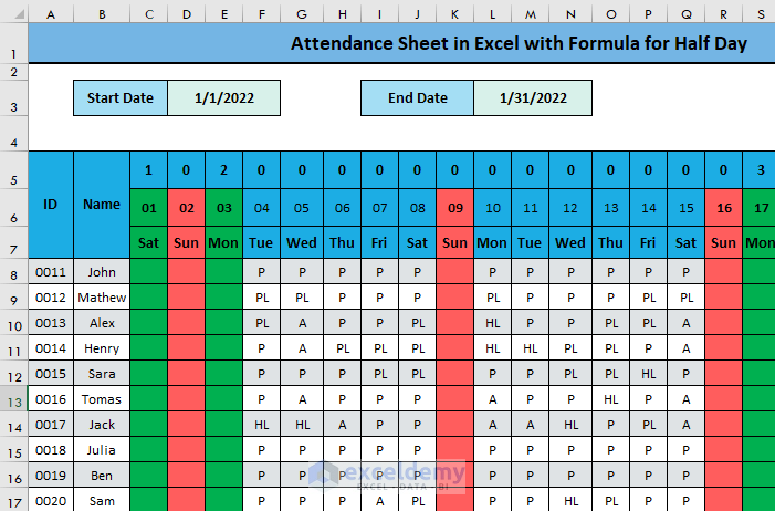
Now, you can calculate the proper count of leaves including the half-day counts using the three formulas given below.
Method 1 – Use COUNTIFS Function
Steps:
- Make a new column for each employee to calculate their total leaves.
- Click on the C5 cell and insert the following formula.
=COUNTIFS('Attendance Sheet'!C8:AG8,"PL")+COUNTIFS('Attendance Sheet'!C8:AG8,"A")+COUNTIFS('Attendance Sheet'!C8:AG8,"HL")/2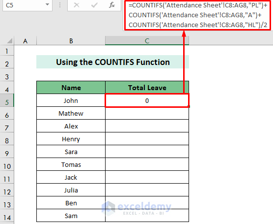
Formula Breakdown:
=COUNTIFS(‘Attendance Sheet’!C8:AG8,”PL”)
This returns you the result of how many “PL” values are there in the range of C8:AG8 cells in the Attendance Sheet worksheet.
Result: 0
COUNTIFS(‘Attendance Sheet’!C8:AG8,”A”)
This returns you the result of how many “A” values are there in the range of C8:AG8 cells in the Attendance Sheet worksheet.
Result: 0
COUNTIFS(‘Attendance Sheet’!C8:AG8,”HL”)/2
This returns the result of how many “HL” values are there in the range of C8:AG8 cells in the Attendance Sheet worksheet. The result is divided by 2.
Result: 0
=COUNTIFS(‘Attendance Sheet’!C8:AG8,”PL”)+COUNTIFS(‘Attendance Sheet’!C8:AG8,”A”)+COUNTIFS(‘Attendance Sheet’!C8:AG8,”HL”)/2
This sums up all the previous breakdown results.
Result: 0
- Hit the Enter button.
- You should see the total leaves of the first employee, John.
- Place your cursor in the bottom right position of C5.
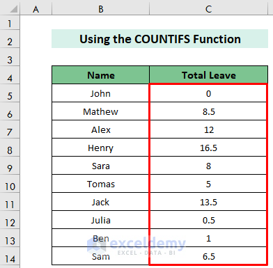
- Drag the Fill Handle downward.
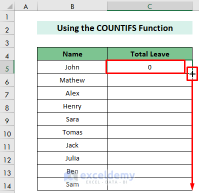
The result would look like this.
Read More: How to Create Employee Attendance Sheet with Time in Excel
Method 2 – Use the SUMPRODUCT Function
Steps:
- Click on the C5 cell.
- Write the following formula in the formula bar.
=SUMPRODUCT(('Attendance Sheet'!C8:AG8="PL")+('Attendance Sheet'!C8:AG8="A")+('Attendance Sheet'!C8:AG8="HL")/2)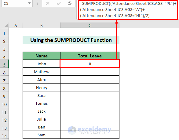
- Press the Enter button.
- You should see the total leaves taken by John.
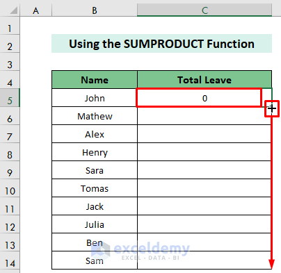
- Place your cursor in the bottom right position of the cell.
- Drag the Fill Handle down to copy the formula to all the other cells below.
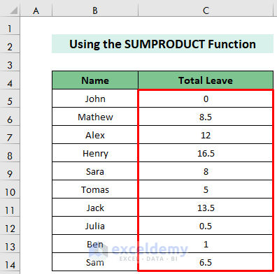
Your output should look like this.
Read More: How to Create a Monthly Staff Attendance Sheet in Excel
Method 3 – Combine the SUM and COUNTIFS Functions
Steps:
- Click on the C5 cell and insert the following formula.
=SUM(COUNTIFS('Attendance Sheet'!C8:AG8,{"PL","A","HL"})*{1,1,0.5})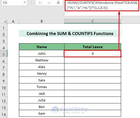
Formula Breakdown:
COUNTIFS(‘Attendance Sheet’!C8:AG8,{“PL”,”A”,”HL”})*{1,1,0.5}
This function finds the “PL”, “A”, and “HL” values in the range of C8:AG8 cells of the Attendance Sheet. Afterward, they multiply the results by 1, 1, and 0.5 respectively.
Result:0,0,0
=SUM(COUNTIFS(‘Attendance Sheet’!C8:AG8,{“PL”,”A”,”HL”})*{1,1,0.5})
This sums up the results got by the COUNTIFS function.
Result: 0
- Hit the Enter button.
- Place your cursor in the bottom right position of the cell.
- Use the black Fill Handle to drag the formula down to the other cells.
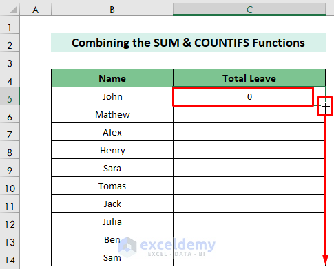
The outcome should look like this.

Read More: Attendance and Overtime Calculation Sheet in Excel
Download Practice Workbook
You can download our practice workbook from here for free!
Related Articles
- How to Create Training Attendance Sheet in Excel
- Labour Attendance Sheet Format in Excel
- How to Create Biometric Attendance Report in Excel
- How to Prepare a Meeting Attendance Sheet in Excel
- How to Create Attendance Sheet with Time in and Out in Excel
- How to Create Monthly Attendance Sheet in Excel with Formula
<< Go Back to Employee Attendance Sheet Excel | Excel HR Templates | Excel Templates
Get FREE Advanced Excel Exercises with Solutions!
