In this article, we’ll describe how to create a meeting attendance sheet in Excel. We’ll assume that an organization holds meetings every day for a month, and prepare a meeting attendance register to record who attended and when.
Step 1 – Making an Information Worksheet
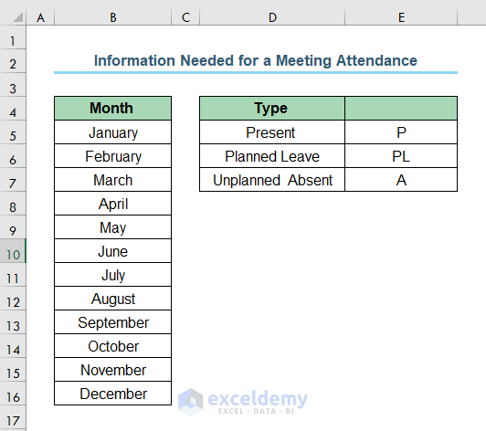
First we need to prepare an information worksheet containing the information necessary to create our meeting worksheet. For purpose of demonstration, we’ve created the following dataset of necessary information named Information Needed for Meeting Attendance. Our meeting attendance will have 12 months and 3 types of activities, namely Present, Planned Leave, and Unplanned Absent.
Step 2 – Defining the Name of Month List
To define the month names in the list:
- Go to Formulas > select the month names in the Month Column > click Define Names.
A New Name window will appear.
- Enter Month for the Name.
- Click OK.
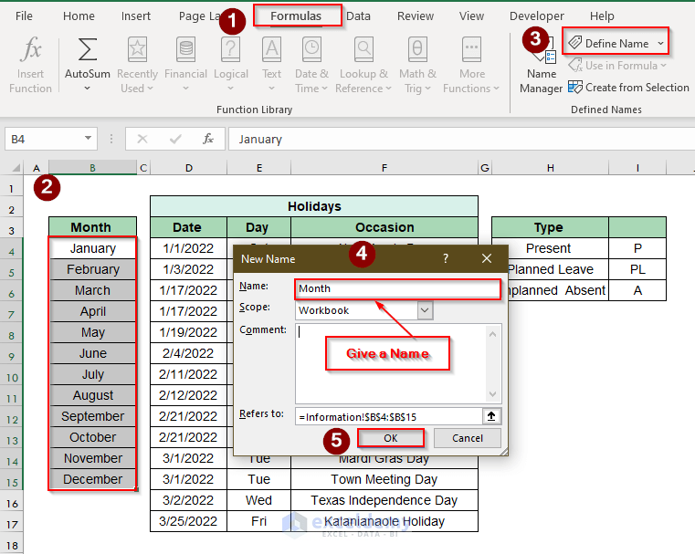
The month names are listed as Month.
To list Type:
- Go to the Formulas tab again > select the Type names in the Type Column > click Define Names.
- In the New Name window, enter Type in the Name box and click OK.
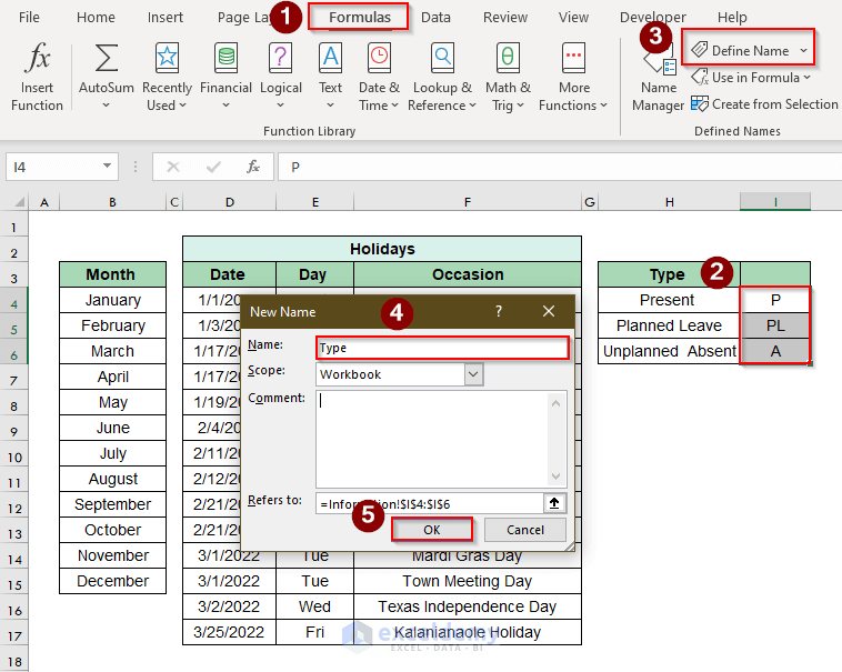
The Type names are also added to a list. We’ll use these two lists to fill validated values in our meeting attendance sheet.
Read More: How to Create Monthly Attendance Sheet in Excel with Formula
Step 3 – Creating the Template Structure
Now we create a template structure which serves as the skeleton of the meeting attendance sheet, and looks like this:.
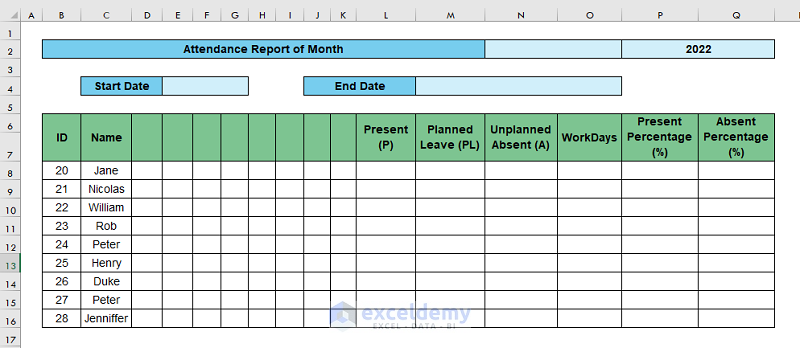
We have added the Start Date and End Date of a month, along with columns to record the Present Percentage and Absent Percentage for each employee in the template.
Step 4 – Inserting Formulas for Month, Start Date and End Date
Next, we insert formulas to fill values for Month, Start Date, and End Date.
- Select cell N2, the Name of the Month.
- Go to the Data tab > select Data Tools > click Data Validation.
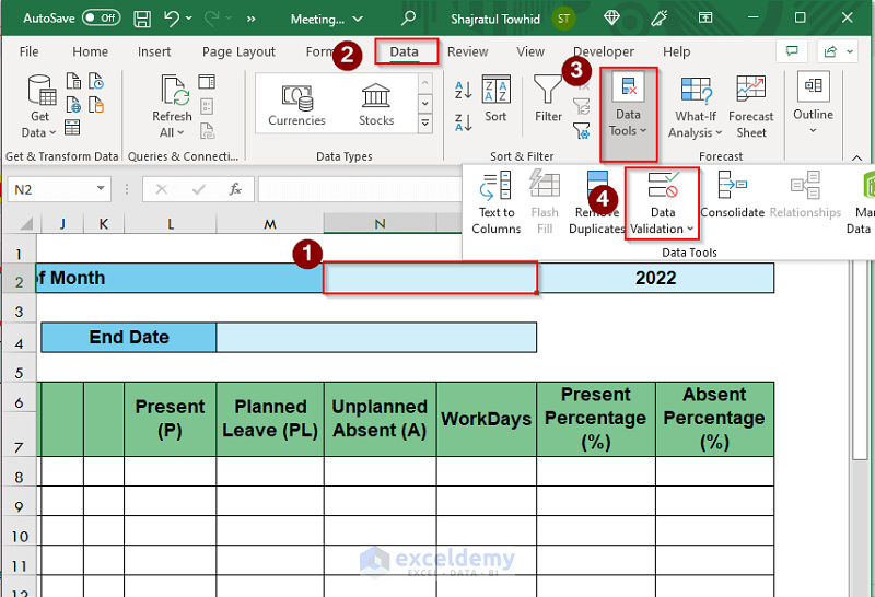
The Data Validation window will appear.
- Go to Settings > select List in the Allow box > type =Month in the Source box > click OK.
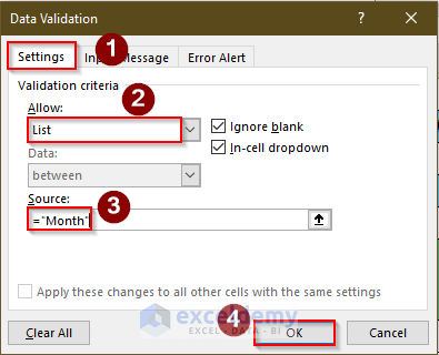
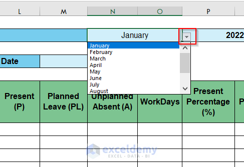
A drop-down bar of months is added in cell N2.
- Now, we’ll set the Start Date and End Date in cells E4 and M4 respectively.
- To set the Start Date, enter the following formula in cell E4:
=DATEVALUE(“1”&N2)
Here, N2 refers to the month name in cell N2. As we are setting the Start Date, we select January as the month name.
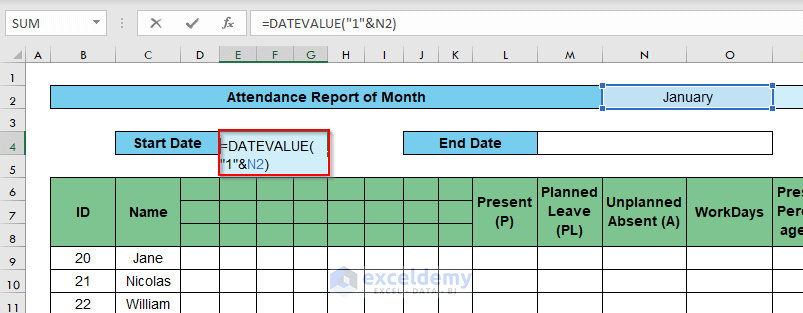
- Press ENTER to return output of 1/1/2022.
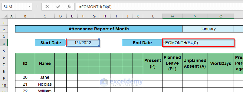
- To set the End Date, enter the following formula in cell M4:
=EOMONTH(E4;0)
Here, E4 refers to the Start Date in cell E4, 1/1/2022.
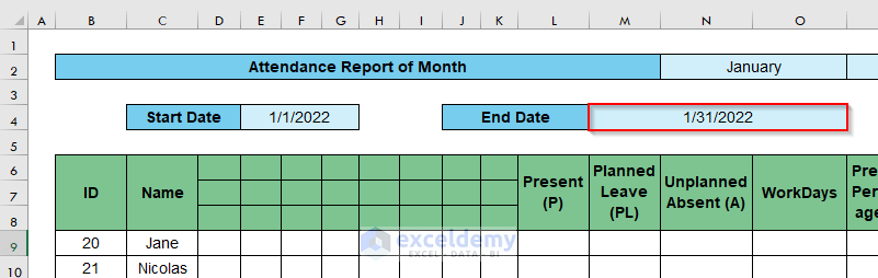
- Press ENTER to return an End Date of 1/31/2022.
Read More: How to Create a Monthly Staff Attendance Sheet in Excel
Step 5 – Entering the Dates
Now we’ll enter the dates in Row 7.
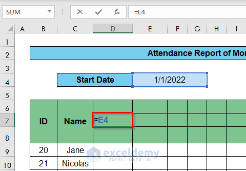
- Enter the following formula in cell D7:
=E4
Here, E4 is the Start Date, i.e. 1/1/2022.
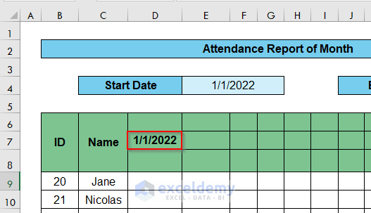
- Press ENTER to return output of 1/1/2022.
We need to change this date format to dd type.
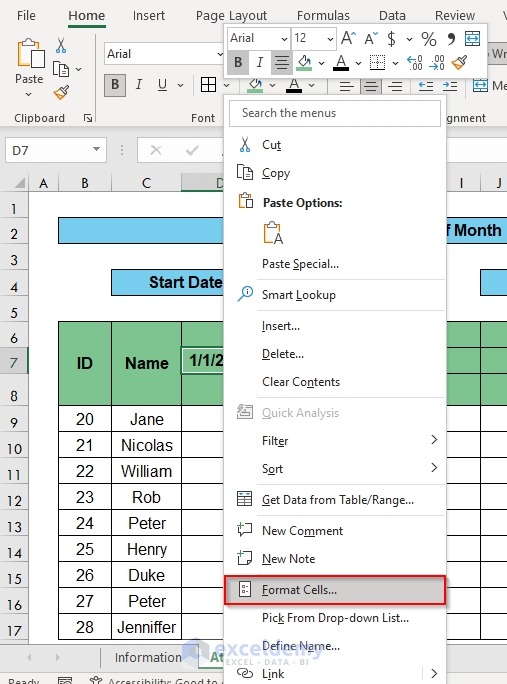
- Right-click on cell D7.
- Select Format Cells from the context menu.
The Format Cells window will appear.
- Go to the Number tab > select Custom > enter dd in the Type box > click OK.
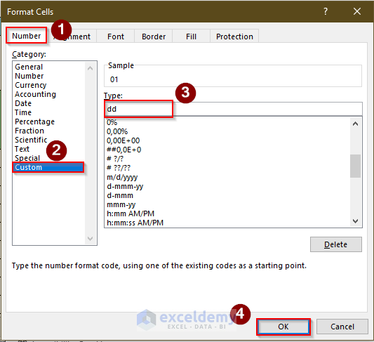
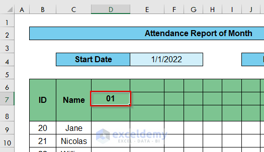
- The output is 01.
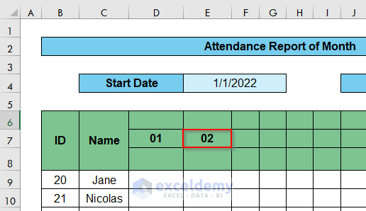
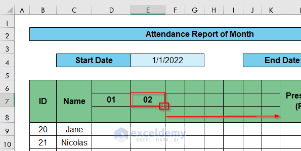
- To set the 2nd date, enter the formula below in cell E7:
=IF(D7<&M&4+1;D7+1;””)
Here, M4 is the End Date.

- Press ENTER to return output of 02.
Note: If the output is again in short date format, change it to dd format by going to Format Cells again.
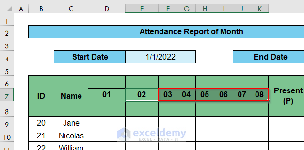
- Use the Fill Handle to copy the formula across to cell K7.
We have dates up to 08.
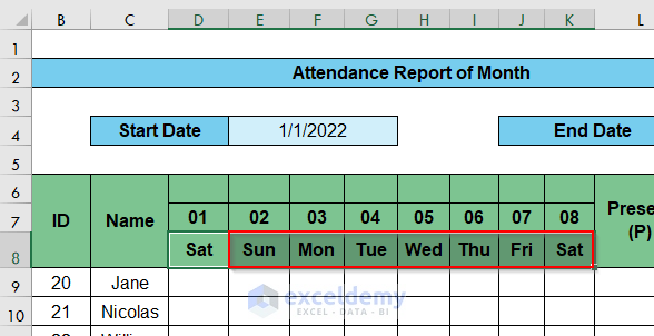
Now, we’ll add week names in Row 8.
- Enter the following formula in cell D8:
=TEXT(D7;”ddd”)Here, D7 is the first date of the month, 01.
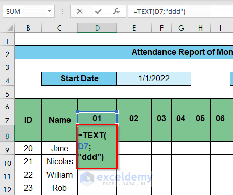
- Press ENTER to return the first day of the week, Saturday i.e. Sat.
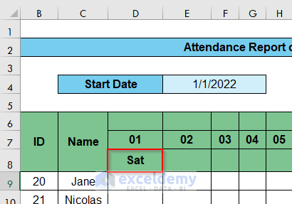
- To get the other days of the week, drag the Fill Handle right.
The output looks like this:
Step 6 – Setting Up a Drop-Down Menu for the Attendance Cells
Next, we’ll set up a drop-down menu for the attendance cells in D9:K28.
- Select the range D9:K28.
- Go to the Data tab > select Data Tools > click Data Validation.

The Data Validation window will appear.
- Click Settings > pick List in the Allow box > write =Type in the Source box > click OK.
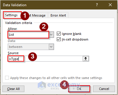
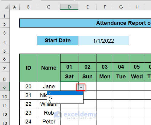
Drop-down bars will appear in every cell of the range D9:K28.
Step 7 – Inserting Data in the Attendance Cells
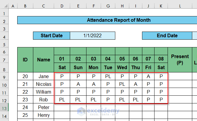
Using the drop-down lists in every cell, fill the attendance sheet with Type values up to Column 12 like in the image below.
Step 8 – Inserting Formulas to Calculate Total Attendance
Now that we have all the raw data, we can work out the number of Present, Planned Leave and Absent days for each of the employees individually. We’ll use the COUNTIF function to find these values.
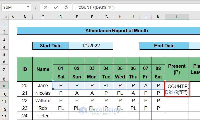
- To calculate the Present days for Jane, enter the following formula in cell L9:
=COUNTIF(D9:K9;"P")
Here, D9:K9 refers to the attendance Type values for Jane.
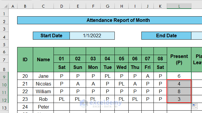
- Press ENTER and use the Fill Handle to get the Present days for Jane and the other employees up to Row 23.
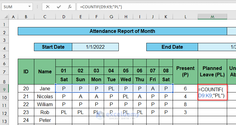
- To calculate the Planned Leave (PL) values, enter the formula below in cell M9:
=COUNTIF(D9:K9;"PL")
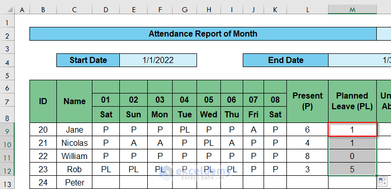
- Press ENTER and use the Fill Handle to get the Planned Leave days for Jane and the other employees.
In the same way, we’ll now find the Unplanned Absent (A) days of the employees.
- Enter the formula below in cell N9:
=COUNTIF(D9:K9;"A")
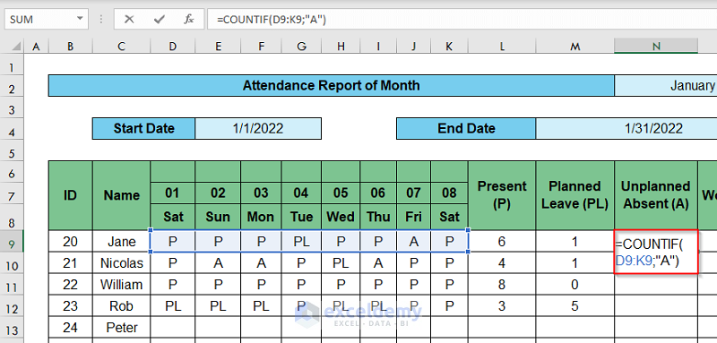
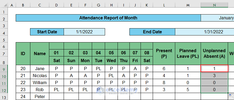
- Press ENTER, and use the Fill Handle to return outputs like this:
We’ll now calculate the Present Percentage of the Employees.
- Enter the following formula in cell O9:
=L9/O9
Here, L9 and 09 refer to the Present days of Jane and Workdays respectively.

- Press ENTER and use the Fill Handle to find the Present Percentage for all the employees.

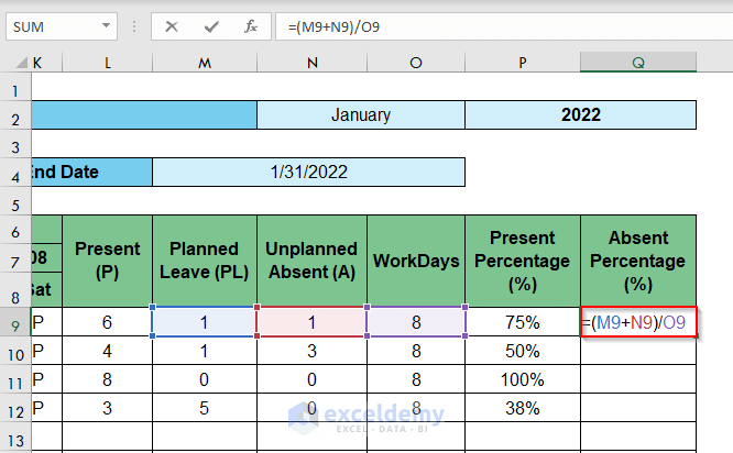
Finally, we’ll calculate the Absent Percentage of the employees.
- Enter the following formula in cell Q9:
=(M9+N9)/O9
Here, M9, N9, and O9 refer to the Planned Leave, Unplanned Absent, and Workdays for Jane respectively.
- Press ENTER and use the Fill Handle to return the Absent Percentage of all the employees.
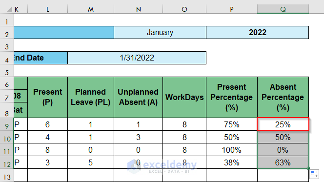
Our meeting attendance sheet is ready to use.
Read More: How to Create Employee Attendance Sheet with Time in Excel
Download Practice Workbook
Related Articles
- How to Create Biometric Attendance Report in Excel
- Labour Attendance Sheet Format in Excel
- Attendance and Overtime Calculation Sheet in Excel
- Attendance Sheet in Excel with Formula for Half Day
- How to Create Training Attendance Sheet in Excel
- How to Create Attendance Sheet with Time in and Out in Excel
<< Go Back to Employee Attendance Sheet Excel | Excel HR Templates | Excel Templates

