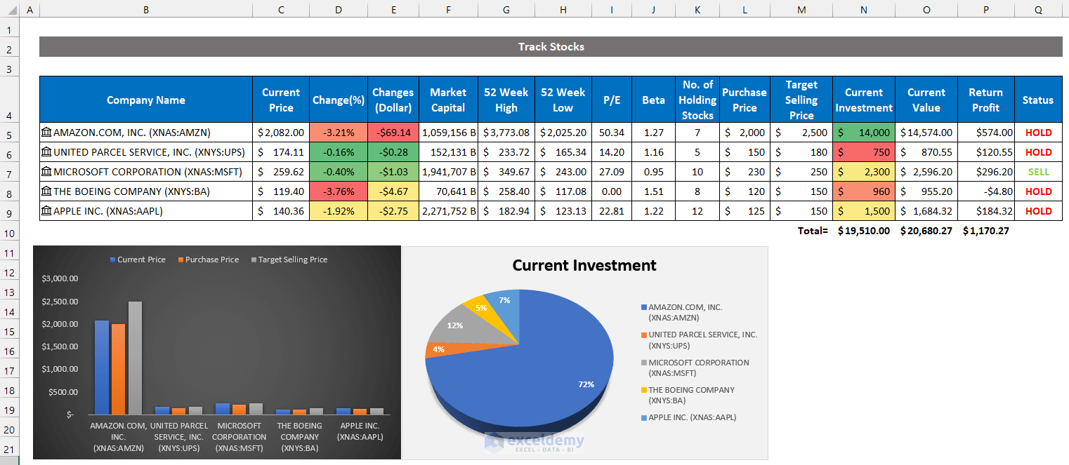
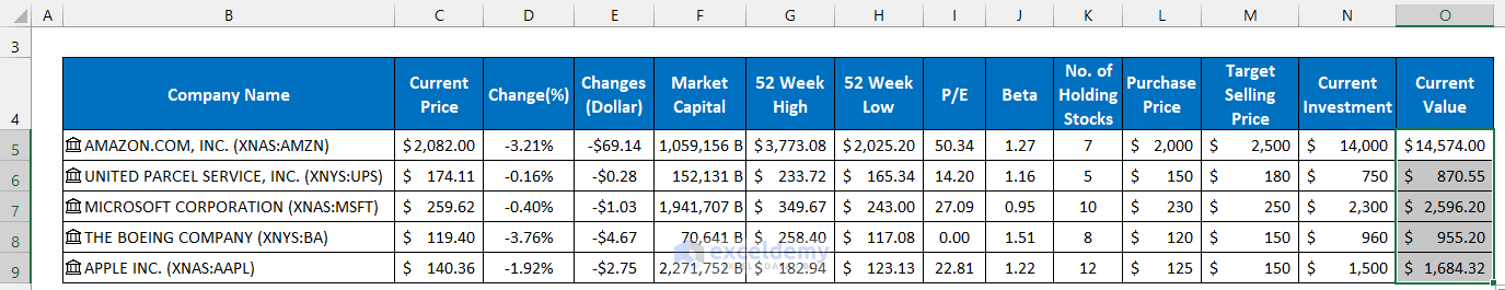
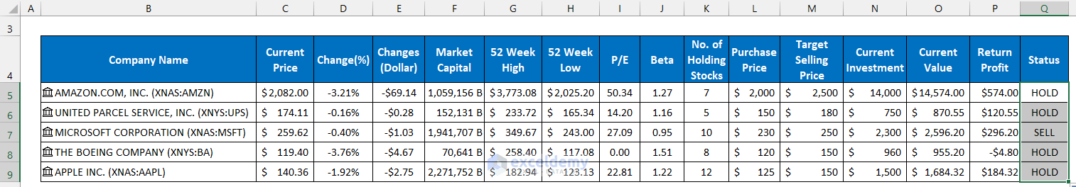
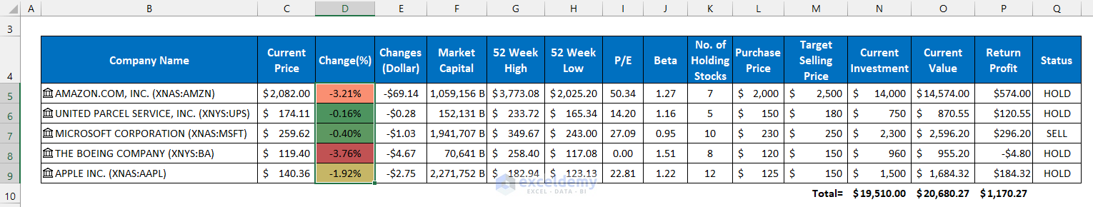
How to Track Stocks in Excel (Download Free Template)

To demonstrate how to track stocks, let’s consider some of the most popular companies in the world, with the names of those companies provided in column B. After completing the stock tracker, it will show as the image.

Step 1 – Inserting Name of Companies in Excel

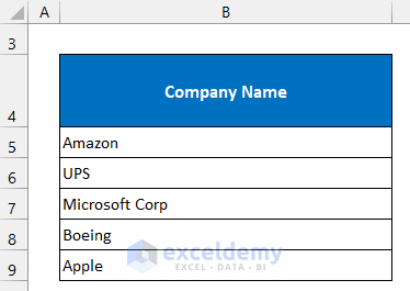
Title column B in cell B4 as Company Name.
Write down your desired company’s names in the range of cells B5:B9. In our dataset, we consider Amazon, UPS, Microsoft Corp, Boeing, and Apple as our desired companies.

Step 2 – Extracting Stocks Information Using Excel’s Built-in Feature

Select the entire range of cells B5:B9.
In the Data tab, select Stocks from the Data Types group.

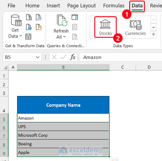
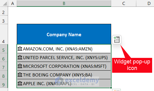
You will see the companies’ name patterns will change, and it will get the complete name structure.
You will see a small widget pop-up icon will appear at the right corner of the selected names.

If you click on it, you will get several fields listed there. We are going to add 8 fields.
Click on the widget pop-up icon, scroll down in the field list with your mouse, and select the Price option.

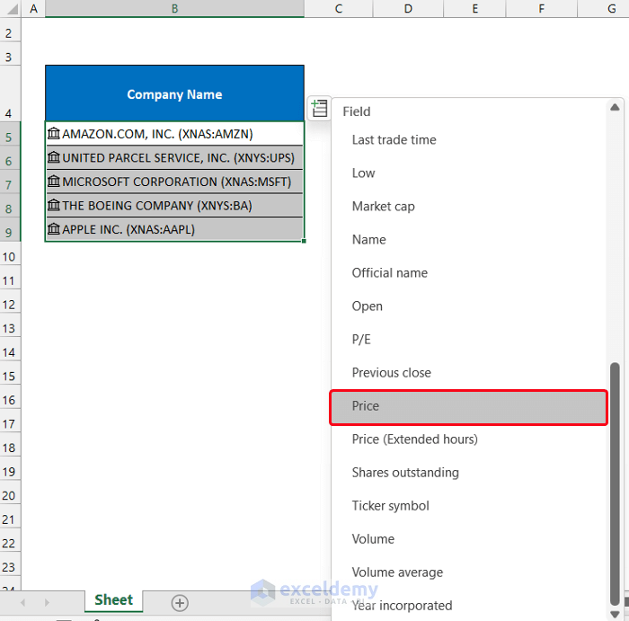
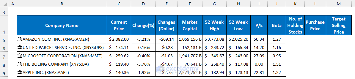
You will see the Price of all five companies added in the range of cells C5:C9.

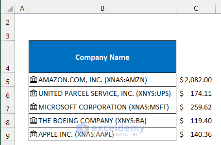
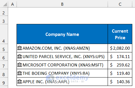
Name the cell C4 as Current Price as the header.

Add the Change (%), Changes, Market cap, 52 Week High, 52 Week Low, P/E, and Beta fields in columns D, E, F, G, H, and I, respectively.
Give the columns their headings.

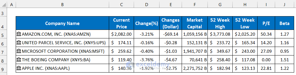
We have completed the second step to track stocks in Excel.

Things You Should Know

The built-in Stock option of Excel’s Data tab provides a live update of the stock price. It usually extracts the information online and shows them here. As a result, when you open the sample template, Excel will automatically refresh the data. If you try create your stock tracker, the values may not match the image on that particular day.

Step 3 – Inserting Our Stocks Information

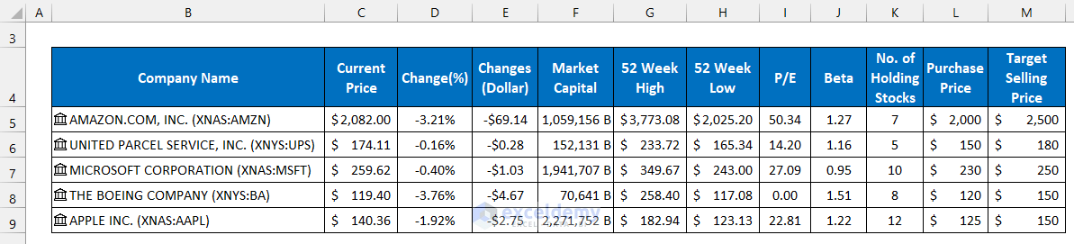
Titled cells K4, L4, and M4 as No. of Holding Stocks, Purchase Price, and Target Selling Price.

Write down the stock amount, their corresponding purchase price, and target selling price.

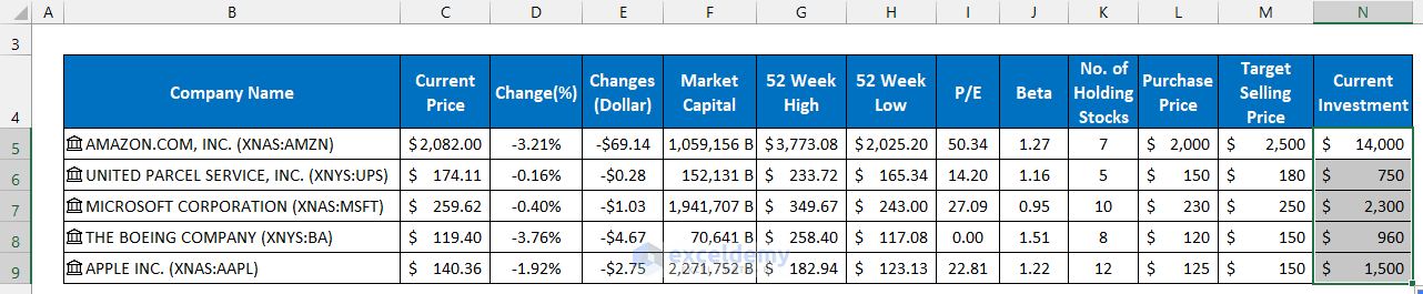
Write down the following formula into cell N5:

=K5*L5

Double-click on the Fill Handle icon to copy the formula up to cell N9.

Step 4 – Tracking Status of Stocks

Set the title in O4 as Current Value and write down the following formula in cell O5:

=C5*K5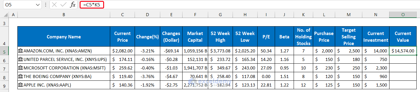

Double-click on the Fill Handle icon to copy the formula up to cell O9.

To get the profit estimate, write down the following formula in cell P5:

=O5-N5

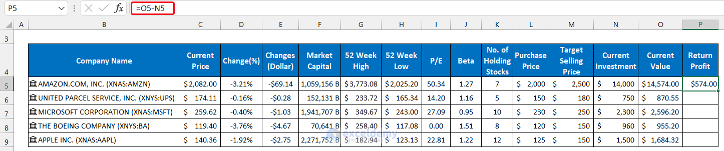
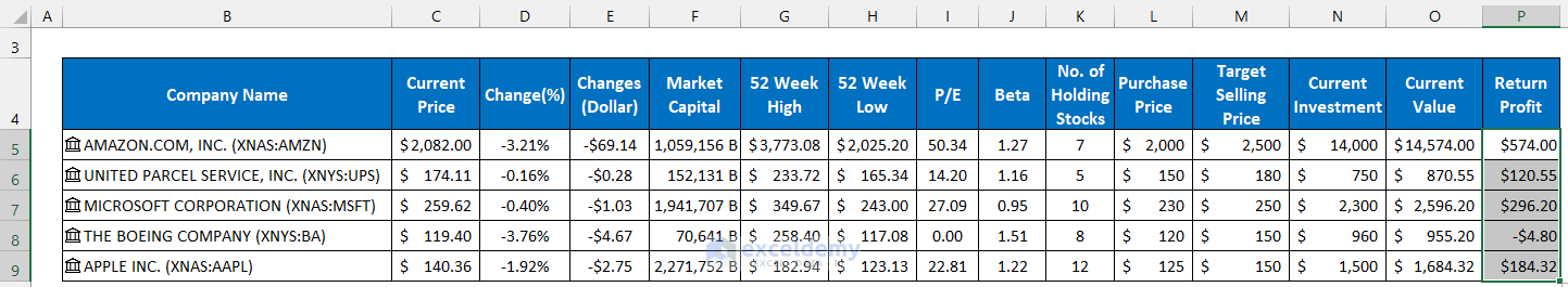
Double-click the Fill Handle icon to copy the formula up to P9.

Write down the following formula into cell Q5:

=IF(C5>M5,"SELL","HOLD")

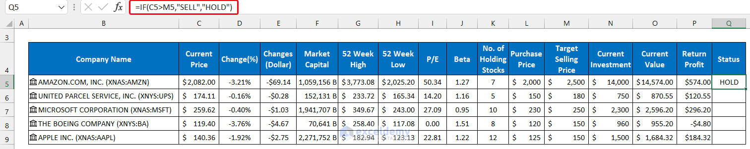
Illustration of the Formula

We are explaining the formula for cell Q5.

The name of the company in row 5 is Amazon. The IF function will check whether the value of C5 (Current Price) is greater than M5 (Target Selling Price). If the test gets a positive result, it will print SELL. Otherwise, the function will return HOLD.

Double-click on the Fill Handle icon to copy the formula up to cell Q9.

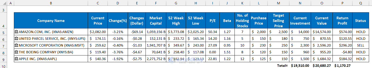
You can also get the total value of your investment, current stock value, and profit using the SUM function.
To calculate the total values, in cell N10, write down the following formula:

=SUM(N5:N9)

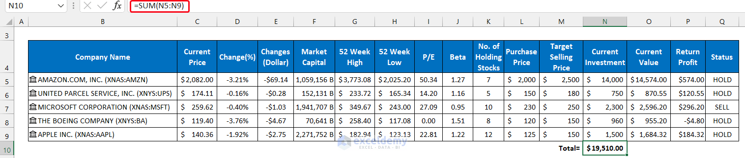
Write down the corresponding formulas for cells O10 and P10 to get their total.

Step 5 – Formatting Key Columns for Better Visualization

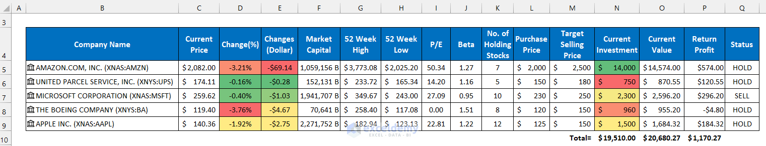
Select the range of cells D5:D9.
In the Home tab, select the drop-down arrow of Conditional Formatting from the Styles group.
Now, select Color Scales and add Green-Yellow-Red Color Scale.

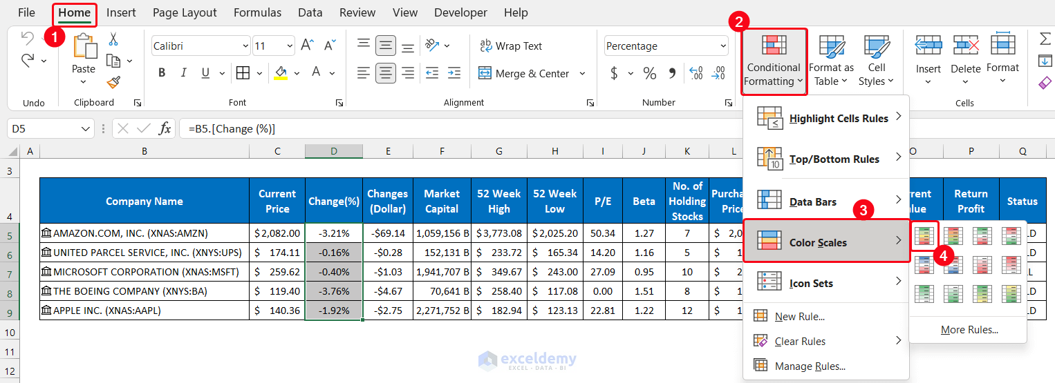
The column’s cells will show in different colors.

Apply the same conditional formatting for columns Changes (Dollar) and Current Investment.

For the Status column, select the range of cells Q5:Q9.
Select the drop-down arrow of Conditional Formatting from the Styles group and choose the New Rule option.

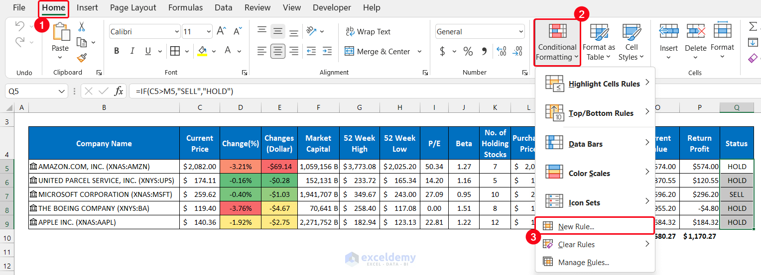
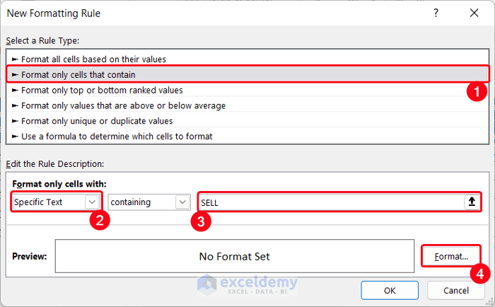
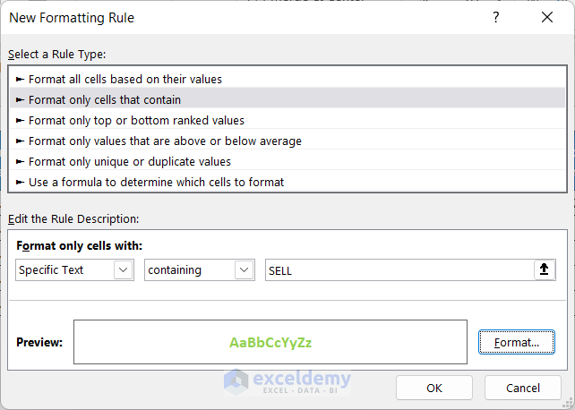
The New Formatting Rule dialog box will appear in front of you.
Select the Format only cells that contain option.
Set the first drop-down box menu as Specific Text and write down SELL in the empty box.
Select the Format option.

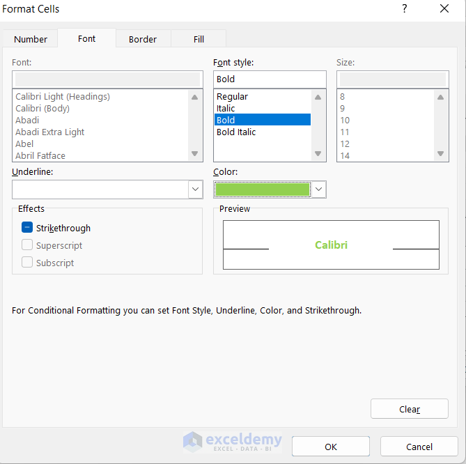
Another dialog box called Format Cells will appear.
Format accordingly. We chose the Font style as Bold and the Color Green.
Click OK.

Click OK to close the New Formatting Rule dialog box.

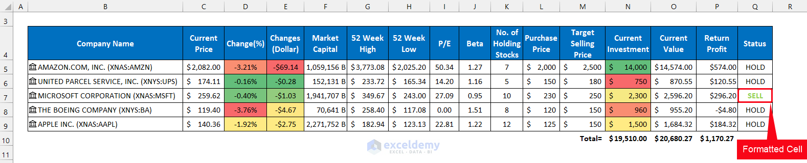
You will see the cell containing SELL showing the formatting.

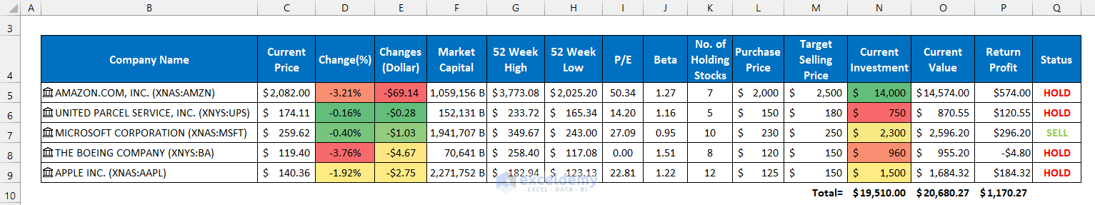
Apply the same type of conditional formatting with a different color for text HOLD.

Step 6 – Inserting Charts to Show Patterns

In the column chart, we will show the Current Price, Purchase Price, and Target Selling Price.
Select the range of cells B4:C9, and L4:M9. (Hold Ctrl while selecting columns to do so).
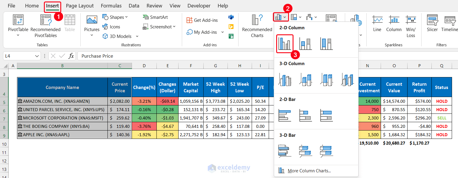
Select the drop-down arrow of the Column or Bar Chart from the Charts group.
Select the Clustered Column option from the 2-D Column section.

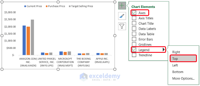
The chart will appear in front of you. Click on the Chart Element icon and check the elements you want to keep. In our case, we checked only the Axes and Legend elements for our convenience. Set the Legend’s position on Top.

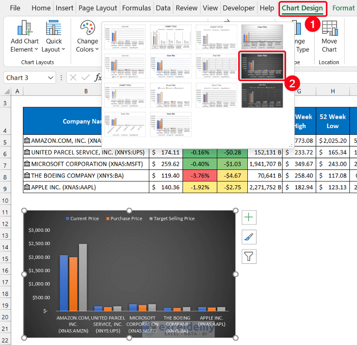
Modify your chart style and texts from the Design and Format tab.
We chose Style 8 for our chart from the Chart Styles group.
Use the Resize icon at the edge of the chart for better visualization.

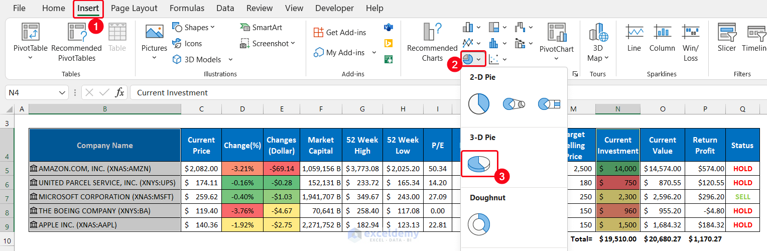
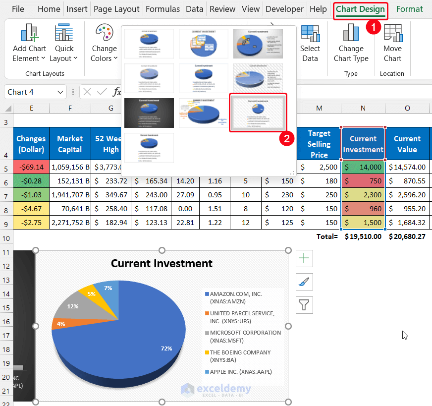
For the Pie chart, select the entire range of cells B4:B9 and N4:N9.
Select the drop-down arrow of the Insert Pie or Doughnut Chart option.
Select the 3-D Pie option.

Adjust the chart style. We chose Style 9 for our chart and checked all the chart elements for the convenience of our chart.

Select the range of cells B2:Q2 and choose the Merge & Center option from the Alignment group.

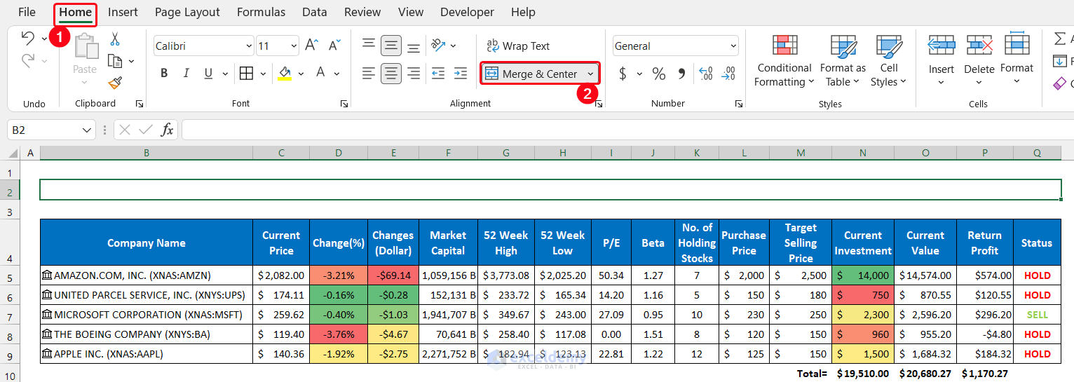
Write down the title for the sheet. We set it as Track Stocks.

Download Template

Download this template which you can use and expand.

Track Stocks.xlsx

<< Go Back to Stocks In Excel| Excel for Finance | Learn Excel

Get FREE Advanced Excel Exercises with Solutions!

10 Comments

Subbaraman Nov 18, 2023 at 11:26 AM

Good work. Can you customize it for Indian stock markets
- Reply
  Lutfor Rahman Shimanto Nov 19, 2023 at 4:19 PM
  
  Hello SUBBARAMAN
  
  Thanks for reaching out and sharing your requirements. Your appreciation means a lot to us. Thanks once again.
  
  You want to analyze the Indian Stock Markets. To achieve your goal, you only need to use the Indian company names, and the rest of the procedure is described in the article.
  
  Like the following GIF, I generated the intended data for some noted Indian Companies.
  
  So, type the Indian company names and follow the steps of this article. Good luck!
  
  Regards
  Lutfor Rahman Shimanto
Varun Feb 19, 2024 at 6:56 PM

Can u provide the same of india stock market with chart as above same in dollars inr instead of $
- Reply
  Lutfor Rahman Shimanto Feb 22, 2024 at 5:16 PM
  Hello VARUN
  
  Thanks for reaching out and sharing your requirements. Your appreciation means a lot to us.
  
  Yes, We can provide information on the Indian stock market with charts in dollars (INR) instead of dollars ($).
  
  You can download this template below for your help. Additionally, I’m also writing down the steps so that you can modify it yourself.
  
  Download Excel file: Track-Indian-Stock-Market.xlsx
  
  Use these steps for indian stock market tracking:
  Add Indian Stock company Names.
  
  Select the range (i.e. B5:B9).
  
  Go to the Data tab > Data Types group > Stocks.
  It will automatically update the Stock Tracker names. However, the values will show an Error Warning.
  
  Select the cell (i.e.C5) > Click the drop-down menu beside the error warning > Click Update format.
  It will automatically update the price in INR format.
  
  Use the Fill handle feature to apply the change in the column.
  Repeat the same process for other columns where necessary till J or Beta Column.
  
  To update the format of Our Stock information section (Column K to P), follow these steps:
  Select the Current Price Column (i.e. B5:B9)
  
  Go to the Home tab > Clipboard group > Format Painter icon.
  
  Select the range (i.e. L5:M9) to apply the format painter. You will notice the paint icon beside the cursor.
  It will apply the same currency format to the applied range. Use the same process for Column O and P.
  
  To update the format with Conditional formatting of Current Investment Column, copy the formatting of Changes (INR) column using Format Painter and paste it. It will automatically update both currency format and conditional formatting.
  
  Note: The charts will update automatically.
  
  Hope this helps you out.
  
  Regards,
  
  Ishrak Khan
  ExcelDemy
Bhavnesh Parikh Feb 26, 2024 at 3:00 PM

Can be available mutul fund scaneer in excel?
- Reply
  Abdullah Al Masud Feb 28, 2024 at 1:08 PM
  
  Hello BHAVNESH PARIKH,
  
  Thank you for reaching out to us and for your valuable query.
  
  While this article focuses on tracking stocks in Excel, you have to modify some of the procedures of this Excel file and include mutual fund data as well.
  
  It is important to mention that, the built-in Stock option of Excel’s Data tab provides us a live update of some major exchanges (like NASDAQ, NYSE, etc.). Popular stock exchanges around the world are easily accessible by this Excel feature, but others are completely unattainable.
  
  To use this stock tracking template for mutual fund scanning purposes, you have to manually collect data on mutual fund names, current prices, 52 Weeks’ High, 52 Weeks’ Low, and P/E ratio. Then use the functions presented in this article for your mutual fund analysis and screening.
  
  Regards,
  Abdullah Al Masud
  ExcelDemy Team
Leo Mulhern Jul 7, 2024 at 6:18 PM

Hi when I try and edit the names of the companies in the spread sheet excel keeps closing itself after the second edit and i cant work out why.
can you help with this?
- Reply
  Shamima Sultana Jul 7, 2024 at 7:59 PM
  
  Hello Leo Mulhern,
  
  The Excel file is working fine in my end. I updated the stocks name and it is working.
  
  Track Stock Prices:
  
  Updated Stock Prices:
  
  Again, I uploaded the Excel file for you:
  Track Stocks in Excel (Updated).xlsx
  
  If new file keeps shutting down, try these steps to fix the issue:
  
  Update Excel: Make sure Excel is up to date.
  Disable Add-Ins: Open Excel in Safe Mode (hold Ctrl while opening Excel), then disable add-ins from File -> Options -> Add-Ins.
  Repair Office: Go to Control Panel -> Programs -> Programs and Features, find Microsoft Office, right-click, select Change, and choose Quick Repair.
  
  Regards
  ExcelDemy
SAQIB HAROON Oct 17, 2024 at 2:17 PM

Can we select Saudi Arabia & Pakistan companies Stock?
- Reply
  Shamima Sultana Oct 17, 2024 at 10:05 PM
  
  Hello Saqib Haroon,
  
  In this article we used Excel’s stocks data to import stocks. Here is the list of Stocks financial data sources.
  Saudi Arabia and Pakistan markets stock prices are not listed in Microsoft Excel stocks. You can use the Yahoo Finance API to get the stock prices if stocks are listed in there.
  
  Regards
  ExcelDemy